While compressor maps are widely referenced in turbomachinery design, the actual generation process—whether through testing or simulation—is often misunderstood or treated as proprietary knowledge. Many engineers use maps without understanding how inlet conditions, corrected parameters, and loss correlations affect accuracy, or how to select between rig testing and computational methods. This guide bridges that gap.
Key Takeaways
- Plot pressure ratio and efficiency vs. corrected mass flow on constant-speed lines from choke to surge
- Build maps from instrumented rig tests or meanline models with validated empirical loss correlations
- Correct flow (× √θ/δ) and speed (/ √θ) so one map holds across ambient conditions via Mach similarity
- Rely on accurate maps for component matching, control-law validation, and surge-margin prediction
- Generate full maps in minutes to hours with tools like SimTurbo—no prototype hardware required
What Is Axial Compressor Map Generation?
Axial compressor map generation is the systematic process of determining and plotting compressor performance parameters—pressure ratio, efficiency, and mass flow—across a range of operating speeds and conditions. The outcome is a performance chart used for engine matching, control system design, and operability analysis from design through field operation.
This process differs from compressor map reading or interpretation, which uses existing maps. Map generation creates new maps from test data on physical rigs or from computational models validated against empirical data.
According to NASA's engine cycle analysis guidelines, a compressor map tabulates total-pressure ratio, corrected flow, and efficiency as functions of corrected speed. That off-design data is what a matched engine cycle requires.
The typical compressor map format includes:
- Horizontal axis: Corrected mass flow (ṁ√θ/δ)
- Vertical axis: Total-pressure ratio
- Curved lines: Constant corrected-speed lines running from choke (right) to surge (left)
- Efficiency contours: Overlaid or tabulated values showing peak efficiency regions
- Surge line: Left boundary connecting the low-flow stability limits
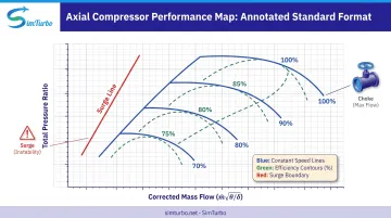
Variable stator or inlet-guide-vane settings may require stacked maps for different geometry configurations, each representing a distinct aerodynamic state.
Why Axial Compressor Map Generation Is Used in Gas Turbine Design
Accurate compressor maps are mandatory for matching compressor, combustor, and turbine components in gas turbine engines to ensure stable operation across flight envelopes or industrial duty cycles. A cycle solver scales the compressor map to the design-point pressure ratio, efficiency, and corrected flow, then iterates to balance shaft work and mass flow between all components. Without this matching capability, engineers cannot predict how the engine will respond to throttle changes, altitude variations, or inlet distortion.
Surge Margins and Safety Boundaries
Maps reveal surge margins and stall boundaries that dictate safe operating limits. Without maps, engines risk compressor surge during transients or off-design operation.
14 CFR 33.65 requires that starting, thrust changes, augmentation, limiting inlet distortion, or inlet temperature not cause surge or stall severe enough to produce flameout, structural failure, overtemperature, or loss of recoverable thrust. Those protections must hold anywhere in the operating envelope.
NASA's engine simulation example showed a low-pressure compressor approaching surge after a 15% thrust reduction and entering surge at deeper throttle-back points. Proximity to the surge line must be monitored continuously.
Consequences of Poor Map Quality
Relying on generic or scaled maps from similar compressors leads to poor performance prediction, missed efficiency targets, and inadequate surge margin in real operation. NASA research on map scaling found that traditional design-point scaling, which preserves the base map's flow-speed relation and applies a pressure-rise scalar, can produce significant component-representation errors.
Interpolation outside tabulated map bounds requires extrapolation and creates problems in matched-cycle solutions.
When Maps Are Required
Map generation is required at multiple stages:
- Early engine design: Component matching and preliminary cycle analysis
- Development phase: Control law validation and transient response tuning
- Post-production: Performance monitoring, diagnostics, and deterioration tracking
- Certification: Airworthiness certification, customer performance guarantees, and OEM cycle-simulation integration
How the Axial Compressor Map Generation Process Works
Compressor maps come from physical rig testing or from computational simulation with meanline or throughflow codes validated against empirical data.
Both paths start the same way: set inlet total pressure and temperature, then lock in geometry—blade angles, annulus areas, tip clearances, and stage count.
Physical Testing Method
Rig setup: The compressor is driven by an electric motor or gas generator, with instrumentation measuring inlet/exit pressures, temperatures, mass flow, and shaft speed at multiple operating points. NASA's W-7 axial-compressor study documented typical instrumentation:
- Inlet total-pressure and total-temperature rakes
- Casing static taps and high-response Kulite pressure transducers
- Blade-row total-pressure probes and temperature sensors
- Exit pressure/temperature rakes and five-hole probes for flow angle
- X-wire probes for velocity components
- V-cone mass-flow device
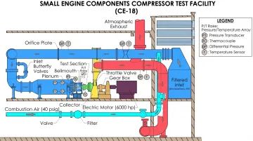
Test procedure: Hold speed at a constant corrected value, then vary back-pressure (throttle valve) from choke to near-surge to trace one speed line. Repeat across multiple speeds so each line runs from maximum flow through peak efficiency to the last stable point before stall.
NASA's testing marks choke, peak-efficiency, and near-stall points on every speed line.
Measurement accuracy: NASA reported the following facility values:
- Inlet static pressure: ±0.015 psi
- Exit static pressure: ±0.03 psi
- Delta-temperature: ±0.5 R
- Efficiency uncertainty: ±0.33 percentage points
- Mass-flow accuracy: ±1.04%
These figures are facility-specific. Actual uncertainty depends on instrumentation quality and should be calculated with ASME PTC 19.1 methods.
Data correction: All measurements are corrected to standard-day conditions with dimensional analysis so the map is not tied to test-day ambient conditions. That correction math is covered in Dimensional Analysis and Corrected Parameters below.
Computational Simulation Method
Modern tools use component-based models with empirical loss correlations (profile, secondary flow, tip leakage) and velocity-triangle calculations to predict stage-by-stage performance.
One-dimensional meanline analysis suits preliminary design. Axisymmetric throughflow methods resolve radial/spanwise redistribution and stage matching at far lower cost than full blade-resolved 3D CFD.
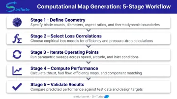
Simulation workflow:
- Define compressor geometry and design point (pressure ratio, efficiency, mass flow, speed)
- Select empirical loss correlations validated for the compressor's Reynolds number and geometry range
- Iterate through speed lines and mass flows, applying conservation equations and loss models at each operating point
- Compute pressure ratio, efficiency, and corrected flow for each speed-flow combination
- Validate predicted choke, peak efficiency, and near-stall behavior against rig data when available
Loss model selection: A 2023 ASME study used an AxS meanline/streamline solver with loss correlations based on Lieblein cascade data. Loss-correlation quality directly affects prediction accuracy—models must account for profile loss, endwall loss, tip leakage, and Reynolds number effects to match real compressor behavior.
Simulation advantages include:
- Map generation in minutes to hours instead of weeks of rig time
- Fast design iterations without building hardware
- Geometry trade studies before any prototype is cut
SimTurbo, for example, uses component-based models with validated loss correlations to build compressor maps in real time for architecture studies and control-law work. Its J85-GE-21 engine simulation stayed within ±2% of NASA test data for thrust, flow rate, temperature, and thrust-specific fuel consumption.
Accuracy still hinges on validation data. Novel blade geometries or operating conditions outside the empirical loss database need physical testing before the map is trusted.
Dimensional Analysis and Corrected Parameters
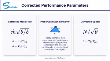
To make maps universally applicable, raw measurements are converted to non-dimensional corrected flow and corrected speed. NASA defines corrected flow using θ = T_t / T_ref and δ = P_t / P_ref (temperature and pressure ratios to standard conditions):
Corrected mass flow: ṁ √θ / δ
Corrected speed: N / √θ
EASA defines corrected rotational speed as N_c = N_r / (T_in / 288)^0.5, giving the familiar N / √θ form.
Corrected parameters absorb ambient swings (altitude, season, ram effects). The same corrected operating point then implies matching Mach numbers and flow angles, even when absolute inlet pressure and temperature change. That preserves velocity-triangle and Mach similarity across test days and flight conditions.
Corrections are not a full free pass. Performance can still shift with:
- Reynolds number and surface roughness
- Tip clearance and heat transfer
- Gas properties and inlet distortion
- Geometry changes and variable-vane schedule
Key Factors That Affect Axial Compressor Map Accuracy
Map accuracy depends on geometry fidelity, loss-model quality, test instrumentation, and off-design incidence behavior. Weakness in any one of these shifts speed lines or moves the surge boundary.
Blade and Vane Geometry Precision
Deviations in stagger angles, chord lengths, or tip clearances from design intent shift speed lines and cut peak efficiency. A 2022 ASME study on manufacturing tolerances found stagger-angle variation mainly affected efficiency and stability boundaries, and recommended smooth circumferential variation rather than abrupt local scatter.
Quality of Empirical Loss Correlations
Simulation accuracy depends on how well profile loss, endwall loss, and tip leakage models match the compressor’s cascade behavior and Reynolds number effects. A 2023 correction method study built adjustments for the coupled effects of Reynolds number, roughness, and tip clearance on a 1.5-stage axial compressor. Those effects cannot be collapsed into a single geometry-only scale factor.
Instrumentation Accuracy in Testing
Pressure, temperature, and mass-flow errors feed straight into efficiency and pressure-ratio calculations, and they grow near surge where gradients are steep. Apply facility-specific uncertainty propagation under ASME PTC 19.1 instead of a generic accuracy band.
Off-Design Incidence Effects
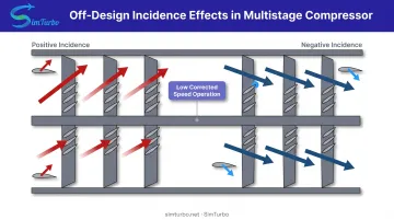
At low corrected speeds, front stages run at positive incidence (toward stall) while rear stages see negative incidence. Accurate angle-dependent loss models are required to place the surge line correctly.
An ASME Turbo Expo 2019 study linked front-stage rotating stall during startup to front/rear-stage operating-point mismatch, and showed that variable-stator-vane angle changes controlled the behavior. NASA’s time-accurate compressor study adds that predicted stall also tracks tip-clearance height, manufactured-vs-design blade geometry, and turbulence modeling—so map boundaries inherit those same sensitivities.
Common Issues and Misconceptions
Even strong map workflows fail when a few common assumptions go unchallenged. These four misconceptions drive most of the avoidable error in axial compressor map generation and use.
Reusing Maps From Similar Compressors
Assuming a compressor map from one engine can be reused on another—without adjusting for Reynolds number, tip clearance, or inlet distortion—produces large errors. NASA found that traditional design-point scaling creates substantial component-representation errors because it keeps the base map's flow-speed relation and never corrects for those physical differences.
Confusing Corrected and Actual Parameters
Operating at "100% corrected speed" does not mean 100% physical RPM when inlet temperature is elevated (for example, high Mach flight). Corrected flow and speed are similarity coordinates, not measured physical quantities.
Both physical and corrected ranges can matter in certification testing. Engineers must convert between them using actual inlet conditions.
Treating Maps as Fixed
Maps shift with compressor deterioration (fouling, erosion) and must be updated for accurate engine performance tracking. A 2014 ASME study modeled fouling as changes to individual axial-stage maps and evaluated part-load degradation and online washing.
Erosion and tip rub change blade geometry, roughness, and clearance, so the map drifts over time. Performance monitoring systems have to track those shifts.
Misinterpreting the Surge Line as a Hard Boundary
Surge is probabilistic. Inlet distortion, transient rates, and manufacturing variability all move the boundary, so safe operation needs margin—not operation right on the surge line.
NASA bracketed the simulated stall point between two throttle settings and showed its location depended on clearance, real-versus-design geometry, and turbulence modeling. The boundary carries inherent uncertainty; retained surge margin (typically 15–25% in normal operation) is the buffer certification and reliable running require.
When Alternative Methods May Not Be Appropriate
Steady-state meanline map generation breaks down when the flow physics fall outside what those models can capture. Use higher-fidelity tools or testing in the cases below.
Highly transient or 3D flow phenomena: Rotating stall cells, tip vortex breakdown, and stall inception need time-accurate CFD, not steady-state meanline maps. A 2024 multistage axial study found full-annulus URANS more appropriate for inherently unsteady flow than steady treatment.
NASA used a full-annulus time-accurate solver and eight circumferential pressure transducers to resolve rotating-stall development, but flagged that approach as resource-intensive.
System surge: A blade-row CFD model without test-facility or engine-system volumes cannot reproduce surge-mode oscillation from ducting and plenum dynamics. NASA noted that full-engine system coupling is required to model these phenomena.
Novel geometries or extreme conditions: Blade geometries or flow conditions far outside the empirical loss-correlation database lack validation, so physical testing becomes necessary. Simulation-based maps still need experimental data inside the compressor's operating regime.
Conclusion
Axial compressor map generation turns compressor geometry and operating conditions into performance charts used for gas turbine design, matching, and control.
Understanding both physical testing and computational simulation helps engineers build reliable maps faster—and read them correctly for safe, efficient operation. Three factors decide whether those maps hold up in practice:
- Corrected parameters keep results comparable across test conditions
- Empirical loss correlations set the accuracy ceiling for simulations
- Proper instrumentation supplies the validation data you need to trust the map
Whether you rely on traditional rig testing or simulation platforms like SimTurbo, accurate compressor maps still drive operability analysis, control system design, and credible performance predictions.
Frequently Asked Questions
What is an axial compressor map?
An axial compressor map is a chart plotting pressure ratio and efficiency against corrected mass flow for various corrected speeds, showing the compressor's performance envelope from choke to surge. Each curved line represents a constant corrected speed, and the left boundary is the surge line marking the stability limit.
How does an axial compressor work?
Rotating blade rows (rotors) add energy to the air by increasing its velocity and angular momentum. Stationary vane rows (stators) convert that velocity into pressure by diffusing the flow and removing swirl. Multiple rotor-stator pairs stack together to form a multistage axial compressor and reach high overall pressure ratios.
How do you read an axial compressor map?
The horizontal axis shows corrected mass flow, the vertical axis shows pressure ratio, and curved lines are constant corrected speed lines. Locate an operating point at the intersection of required flow and speed, then check proximity to the surge line for stability margin and read efficiency from nearby contours.