The stakes are high. An Air Force Research Laboratory (AFRL) review identified combustion-dynamics prediction as a critical design capability, noting that sophisticated Large Eddy Simulation (LES) and data from Direct Numerical Simulation (DNS) are essential for propulsion-component development. The challenge is balancing chemical complexity, turbulence effects, and computational efficiency in simulations that inform billion-dollar propulsion systems, power plants, and industrial processes.
This guide explores how combustion models work, compares the major model families, and provides a practical framework for selecting the right approach based on your application, required outputs, and computational resources.
Key Takeaways
- Combustion models collapse hundreds of species and reactions into tractable frameworks via mixing, rate, and turbulence-chemistry assumptions
- Flamelet/tabulated models run nearly 11x faster than detailed chemistry by using pre-calculated lookup tables
- Pick models by combustion regime, required outputs (heat release vs pollutants/extinction), and computational budget
- Wrong turbulence-chemistry closures can produce species differences exceeding 50% in validation cases
- Platforms like SimTurbo enable component-based combustor modeling for real-time gas turbine work without heavy CFD cost
What Are Combustion Models?
Combustion models are mathematical frameworks that predict fuel-oxidizer reactions, heat release, and species evolution within CFD simulations. They bridge conservation equations for mass, momentum, and energy with thermodynamics, molecular transport, and chemical source terms.
The core challenge: combustion involves hundreds of chemical species and reactions across vastly different timescales. The widely used GRI-Mech 3.0 mechanism for methane, for example, contains 53 species and 325 reactions.
A 2021 review placed the practical ceiling for LES at 20–30 species and 80–100 reactions, so reduction or tabulation is almost always required before embedding detailed chemistry in multidimensional simulations.
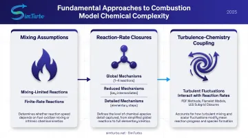
Models handle that complexity in three ways:
- Mixing assumptions – Models distinguish between mixing-limited (infinitely fast chemistry) and finite-rate (slower, kinetically controlled) reactions
- Reaction-rate closures – Global mechanisms use 1–4 overall reactions, reduced mechanisms retain key intermediates, and detailed mechanisms track elementary steps
- Turbulence-chemistry coupling – Models must account for how turbulent fluctuations interact with nonlinear reaction rates
Fundamental Combustion Regimes
Premixed combustion: Fuel and oxidizer are thoroughly mixed before ignition. The flame front separates unburnt from burnt zones, and models typically track a progress variable ranging from 0 (fresh mixture) to 1 (fully burned). Common in lean-burn gas turbines and spark-ignition engines.
Non-premixed (diffusion) combustion: Fuel and oxidizer enter the combustion chamber separately and mix as they burn. The mixture fraction—a conserved scalar representing the fuel stream's mass fraction—naturally parameterizes diffusion flames. Typical in diesel engines, industrial burners, and many rocket combustors.
Partially premixed combustion: Both mixture fraction and reaction progress vary spatially, creating zones with both premixed and diffusion-flame characteristics. Requires hybrid models that can handle mixed regimes.
Chemical Kinetics Mechanisms: Balancing Detail and Cost
| Mechanism Level | Content | Selection Implication |
|---|---|---|
| Detailed | Elementary reactions and intermediate species; GRI-Mech 3.0: 53 species/325 reactions | Highest chemical fidelity; usually too large for direct multidimensional LES |
| Reduced/Skeletal | Removes species/reactions while preserving flame speed, ignition delay, and extinction strain rate | Match reduction targets to required CFD predictions |
| Global | 1–4 overall reactions; tuned for heat release and major species | Appropriate for bulk energy release; unsuitable for ignition, extinction, or pollutants unless specifically validated |
Reduced methane mechanisms require approximately 5% of the GRI-Mech 3.0 simulation time in one-dimensional comparisons, illustrating the direct cost-fidelity trade-off.
Key Types of Combustion Models
Eddy Dissipation Model (EDM) and Eddy Dissipation Concept (EDC)
Eddy Dissipation Model (EDM): The foundational Magnussen-Hjertager closure assumes chemistry is infinitely fast and controlled purely by turbulent mixing. EDM makes the mean reaction rate proportional to turbulent eddy dissipation and limiting-reactant availability. It is an algebraic, mixing-limited model for cases where chemical time is far shorter than mixing time.
When to use EDM: Use EDM for high-temperature, fast-reacting turbulent systems where mixing is the bottleneck, such as industrial furnaces or well-mixed gas turbine combustors operating far from extinction limits.
Eddy Dissipation Concept (EDC): EDC extends the framework by splitting each computational cell into reacting fine structures and non-reacting surroundings. Detailed chemical kinetics are evaluated in reactor-like fine structures (modeled as perfectly stirred or plug-flow reactors), and the mean source term becomes a mass-transfer rate between zones. This allows EDC to handle finite-rate chemistry effects.
When to use EDC: Use EDC when pollutant formation (NOx, CO, soot) or slow chemistry steps (ignition delay, extinction) matter.
EDC’s documented assumptions include:
- Fully developed turbulence
- Cell dimensions larger than flame-reaction-zone thickness
- Exclusion of laminar or near-laminar combustion
Sensitivity caution: Different EDC fine-structure treatments produced species differences exceeding 50% and temperature differences up to 10% in Sandia Flame D validation cases. Always validate the exact closure implementation, not just the model-family name.
Non-Premixed (PDF/Flamelet) Models
Non-premixed models use pre-calculated lookup tables (flamelet libraries) instead of solving transport equations for every chemical species during the CFD run. The flamelet approach precomputes lower-dimensional laminar-flame states, then retrieves thermochemistry through control variables such as mixture fraction, scalar dissipation rate, and progress variable.
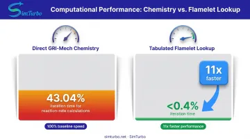
Computational advantage: Jha and Groth (University of Toronto, 2011) found tabulated schemes ran nearly 11x faster than direct GRI-Mech chemistry integration. Reaction-rate calculations consumed 43.04% of iteration time with direct chemistry versus <0.4% with table lookup.
Cost-accuracy trade-off: In an aero-engine LES comparison (Karalus et al., 2022), clustered detailed chemistry cost about 4x more than Flamelet Generated Manifold (FGM) but predicted smoke number more accurately. The optimal choice depends on whether the target output requires fine chemical resolution or whether heat release and major species suffice.
Mixture fraction concept: Mixture fraction is a conserved scalar representing the local mass fraction originating from the fuel stream. That reduces the problem from tracking dozens of species to one or two control variables. Computational cost drops sharply, while the pre-calculated flamelet library still carries realistic chemistry effects.
Premixed Combustion Models
Premixed models track the flame front using a progress variable (c-equation) that ranges from 0 (unburnt mixture) to 1 (fully burnt products). The progress variable is transported with convection, diffusion, and a modeled combustion source term. One common definition uses normalized CO plus CO₂ mass fraction as the progress variable for methane-air flames.
Application fit:
- Lean-burn gas turbines where fuel and air are premixed upstream
- Spark-ignition engines
- LES cases where flame position, surface area, and burning rate are more critical than resolving every elementary reaction step
Premixed models work well when the Karlovitz and Damköhler numbers confirm the flame operates in a regime where the turbulent flame-brush concept is valid.
Partially Premixed Models
Partially premixed environments exhibit both premixed and non-premixed zones, so a single flamelet manifold may fail. Flamelet Generated Manifold (FGM) addresses this by projecting unsteady species equations onto a restricted composition space. One five-dimensional FGM formulation used two composition directions and three scalar-dissipation rates to capture the hybrid behavior.
When to use FGM:
- Stratified-charge engines
- Lifted flames with both premixed and diffusion zones
- Any combustor where mixture fraction and progress variable both vary significantly
Limitation: Purely premixed flamelet tables can fail in rich, partially premixed, or diffusion-controlled regions where fluxes across mixture-fraction surfaces dominate. Check that your FGM table coordinates span the full composition space your combustor will encounter.
Species Transport and Finite Rate Chemistry
The species transport approach solves an individual conservation equation for each chemical species, including convection, molecular/turbulent diffusion, and chemical production or destruction. Species mass fractions couple back to mixture properties and energy, creating a tightly integrated system.
When this detailed approach is necessary:
- Complex fuels (jet fuel surrogates, biofuels) requiring multicomponent chemistry
- Pollutant prediction (NOx, CO, unburned hydrocarbons, soot precursors)
- Slow chemistry regimes (ignition delay, flame extinction, cool flames)
- Cases where tabulated manifolds cannot capture the required physics
Computational cost trade-off: Stiff nonlinear chemistry ODEs must be integrated in every reacting cell at every time step. Implicit solvers add Jacobian construction and factorization overhead. One benchmark showed that three reduced methane mechanisms required about 5% of the GRI-Mech 3.0 simulation time in one-dimensional tests, showing direct scaling with mechanism size.
Chemistry reduction techniques: Reduction methods preserve selected targets (flame speed, ignition delay, extinction strain rate) over the intended operating envelope. Validate all three targets across the full range of temperatures, pressures, and equivalence ratios your simulation will encounter. CHEMKIN-format files provide a standard mechanism input but do not guarantee the mechanism is valid for your specific application envelope.
Turbulence-Chemistry Interaction Models
Turbulent fluctuations cannot be ignored in combustion modeling because chemical reaction rates are highly nonlinear functions of temperature and concentration. Averaging or filtering these nonlinear source terms creates unclosed correlations: reaction rates evaluated from mean temperature and composition generally do not equal the mean of instantaneous rates.
Fundamental TCI Approaches
| TCI Approach | Mathematical Treatment | Main Trade-off |
|---|---|---|
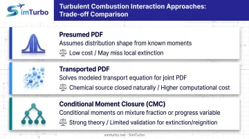
| Presumed PDF | Assumes a probability density function shape (often beta or clipped Gaussian) from known moments like mean and variance | Low computational cost; may miss local extinction if the assumed distribution doesn't match reality |
| Transported PDF | Solves a modeled transport equation for the joint one-point, one-time PDF of composition and enthalpy | Chemical source is closed naturally; micromixing and transport closures plus stochastic particle methods raise cost significantly |
| Conditional Moment Closure (CMC) | Solves conditional moments of species/enthalpy conditioned on mixture fraction or progress variable | Strong theoretical foundation; 1999 review noted validation remained limited for strong local extinction/reignition |
Practical implication: Models that ignore turbulence-chemistry interaction can overpredict or underpredict reaction rates and flame stability. In Sandia Flame D, alternative EDC fine-structure treatments (different TCI closures within the same model family) produced species differences above 50% and temperature differences up to 10%. Validate the exact closure implementation, not just the model-family name.
Presumed PDF sensitivity: An extended Flamelet Progress Variable (FPV) model used a presumed PDF constrained by mixture-fraction and progress-variable moments. A delta-function closure (no fluctuations) underpredicted extinction in Sandia flames; more realistic PDF shapes improved accuracy.
Selecting the Right Combustion Model for Your Application
Choose a combustion model by balancing required outputs, combustion regime, and compute budget. Use this four-step framework:
Step 1: Identify Your Combustion Regime
- Premixed: Fuel and oxidizer mixed before ignition → progress-variable models, G-equation, or flame-surface-density closures
- Non-premixed: Fuel and oxidizer enter separately → flamelet/FPV with mixture fraction and scalar dissipation
- Partially premixed: Both regimes coexist → multidimensional FGM or hybrid models
Step 2: Assess Chemistry Speed
Is chemistry fast (mixing-limited)?
- Yes → EDM or simple flamelet models
- No → Finite-rate kinetics required (EDC, species transport, or transported PDF)
Validation requirement: If finite-rate effects matter, confirm your mechanism is validated for flame speed, ignition delay, and extinction strain rate over your full operating envelope (temperature, pressure, equivalence ratio).
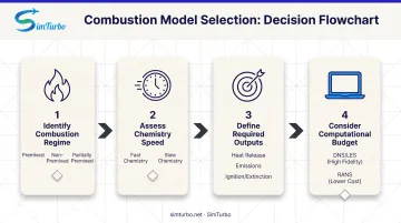
Step 3: Define Required Outputs
| Required Output | Recommended Model Family |
|---|---|
| Bulk heat release and major species | EDM with global chemistry; simple flamelet |
| Temperature field and thrust | Flamelet/FPV; EDC with reduced chemistry |
| NOx, CO, soot, or UHC emissions | Finite-rate species transport; EDC with detailed kinetics; transported PDF |
| Ignition delay and extinction limits | Reduced finite-rate species transport; CMC; transported PDF |
| Combustion dynamics and instability | LES with validated TCI closure; explicit sensitivity analysis |
Step 4: Consider Computational Budget
DNS/LES approaches: Resolve turbulent scales down to or near the reaction zone. Require fine grids, small time steps, and significant CPU/GPU resources. Best suited for research, validation database generation, and high-fidelity design studies.
RANS with combustion models: Model all turbulent scales. Lower cost, faster turnaround. Appropriate for design-space exploration, parametric studies, and cases where time-averaged statistics suffice.
Hybrid and real-time platforms: When full CFD is too costly, component-based engine simulators bridge the gap. SimTurbo models combustion chambers within a real-time gas turbine system so you can study transient performance, controls integration, and cycle behavior on a standard PC.
Against NASA Lewis J85-GE-21 test data, SimTurbo matched thrust, flow rate, temperature, and TSFC within ±2%—useful accuracy for system-level trade studies before you commit to high-fidelity CFD.
Industry-Specific Considerations
Budget and fidelity targets shift by sector:
Aerospace (high pressure, fast reactions):
- Prefer models validated at elevated pressures
- Fast chemistry often supports mixing-limited options (EDM, simple flamelet)
- Dynamics and altitude relight still need LES with validated closures
Power generation (NOx prediction critical):
- Finite-rate chemistry is essential for pollutant formation
- Longer residence times and lower temperatures favor detailed kinetics
- Use EDC or species transport with validated NOx mechanisms
Automotive (transient conditions):
- Capture ignition, combustion phasing, and load transients
- Direct-injection engines often need partially premixed models
- Control development usually requires real-time or near-real-time solvers
Validation and Credibility Framework
Before you lock a model, separate two checks:
- Verification (NASA/AIAA): Confirm the numerics solve the intended equations correctly
- Validation: Confirm those equations represent the physics across your operating envelope
Screen tabulated closures with published flamelet regime diagrams (grid scale vs. reaction-zone thickness and the flamelet-regime parameter). Confirm the regime fits before you adopt the table, then run sensitivity cases on closure constants and submodel choices so the CFD can support design decisions with defensible uncertainty bounds.
Emerging Trends in Combustion Modeling
Machine learning is changing how combustion models handle stiff chemistry and turbulence–chemistry closure. Three directions matter most for propulsion and gas-turbine simulation.
Machine Learning for Chemistry Acceleration
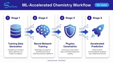
Artificial neural networks (ANNs) accelerate chemistry tabulation while keeping physical constraints intact. A 2021 study (Ding et al.) trained multilayer perceptrons on hybrid flamelet/random training data and reported a 12x reaction-step speedup with close agreement to direct integration. The networks serve as chemistry accelerators that still obey conservation laws.
ML-accelerated chemistry tables can reach near-detailed-kinetics accuracy at flamelet-like cost when training data covers the simulation’s operating envelope and out-of-sample validation is rigorous.
Hybrid Physics-ML Approaches
A 2022 review grouped ML combustion-modeling work into chemical-kinetics acceleration, reduced representations, and subgrid combustion closure. The strongest practical path pairs first-principles models with learned corrections for turbulence-chemistry closure.
Researchers train reduced or subfilter models on high-fidelity DNS or LES data, then embed them inside resolved LES rather than replacing the conservation equations. The Air Force Research Laboratory (AFRL) identifies this multiscale hybrid approach as a priority for propulsion components.
Dynamics-Informed Reduced-Order Models
A 2024 encode-forecast-decode framework pairs a nonlinear autoencoder with a neural ordinary differential equation (ODE) solver for stiff chemistry. It learns a reduced latent space where chemistry integration is faster and more stable, then decodes back to full composition space.
Why it matters: ROM methods can support real-time or near-real-time combustion simulation for control-system design, hardware-in-the-loop testing, and virtual prototyping without dropping essential chemical detail.
Frequently Asked Questions
What is the combustion method?
Combustion is a chemical oxidation process that releases energy rapidly enough to produce heat and often light. In engineering, "combustion method" means the mathematical framework used to model that process in CFD, such as flamelet, species transport, or eddy dissipation approaches.
What are three types of combustion?
The three primary types from an engineering modeling perspective are premixed (fuel and oxidizer mixed before ignition), non-premixed or diffusion (fuel and oxidizer enter separately and mix as they burn), and partially premixed (regions with both premixed and diffusion-flame characteristics).
What are 5 examples of combustion?
Engineering combustion applications include gas turbine engines (aircraft and power generation), rocket combustors, internal combustion engines (automotive and marine), industrial furnaces (steel, glass, cement), and power plant boilers (coal, natural gas, biomass).
What is the difference between a combustion model and a chemical kinetics mechanism?
A chemical kinetics mechanism defines the detailed chemistry: species, elementary reactions, and rate constants. A combustion model couples that chemistry with fluid flow, turbulence, heat transfer, and transport in CFD (for example, flamelet, EDC, or species transport).
How do I choose between premixed and non-premixed combustion models?
Choose based on how fuel and oxidizer enter the chamber. Use a premixed model when they mix upstream before ignition (lean-premixed gas turbines, spark-ignition engines). Use a non-premixed model when they enter separately and burn at the mixing interface (diesel engines, many industrial burners).
What role does turbulence play in combustion modeling?
Turbulence sets mixing rates and creates local swings in temperature and concentration that strongly change reaction rates. Because those rates are nonlinear, models need turbulence-chemistry interaction closures or heat release, emissions, and flame stability predictions can be badly wrong.