Introduction
Control engineers know the challenge all too well: manually tuning PID controllers through trial-and-error can consume days of work, especially on gas turbine engines with complex, nonlinear dynamics.
Each gain adjustment needs a test run. Each run produces new data that must be interpreted while you balance response speed, stability margins, and disturbance rejection.
PID autotuning automates that process. It injects test signals into the plant, measures the response, and calculates optimal proportional (Kp), integral (Ki), and derivative (Kd) gains with established algorithms. You cut engineering time and get more consistent performance. In documented multicopter flight-control testing, adaptive autotuning achieved 38.4% lower simulation cost and 32.3% lower physical-flight cost versus default parameters.
This article covers how PID autotuning works, from Ziegler-Nichols to model-based methods, and how simulation platforms support safe controller validation. On gas turbines, control-law errors can cause compressor stall, temperature excursions, or catastrophic failure—so validating gains before hardware tests matters.
Key Takeaways
- PID autotuning calculates gains from plant tests and algorithms—no manual trial-and-error
- Pick the method to fit the plant: Ziegler-Nichols, AMIGO, model-based, or optimization-based
- Run closed-loop to keep stability, or open-loop only on plants that are already stable
- Gas turbines need gain checks across the full envelope—nonlinear dynamics shift with operating point
- Simulate first: validate PID gains safely before any hardware implementation
What is PID Autotuning?
PID autotuning is an automated process that determines optimal controller gains—proportional (Kp), integral (Ki), and derivative (Kd)—by systematically analyzing how a plant responds to test inputs.
Instead of manually adjusting gains through trial and error, autotuning algorithms inject controlled signals, measure the response, estimate system characteristics, and calculate gains that meet specified performance criteria.
Manual tuning demands domain expertise, burns engineering time, and often yields inconsistent results. Engineers must balance competing objectives: fast response versus minimal overshoot, tight tracking versus disturbance rejection, and aggressive performance versus robust stability margins. Autotuning turns those tradeoffs into algorithmic rules.
Two main approaches exist:
- Closed-loop autotuning keeps an initial stabilizing controller active during frequency-response or relay tests, so the plant stays under regulation with minimal disruption
- Open-loop autotuning disables feedback and applies step or sinusoidal inputs directly to the plant—cleaner identification signals, but only for stable plants and at the cost of interrupting normal operation
Key tuning objectives include:
- Keep the closed-loop system stable across expected operating conditions
- Hit rise time, settling time, and tracking accuracy targets
- Hold phase margin (typically 45–60°) and gain margin high enough to tolerate modeling errors, parameter drift, and disturbances
These margins are context-specific. MathWorks' PID autotuning implementation defaults to 60° phase margin, while documented motor-drive applications report using phase margins between 30-60°. The goal is not a universal number, but consistent, validated controller behavior for your application.
How PID Autotuning Works
The general autotuning workflow follows four steps:
- Inject test signals into the plant
- Measure the response
- Estimate system characteristics
- Calculate optimal gains based on performance criteria
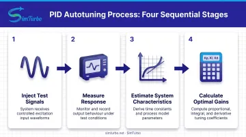
Signals, estimation methods, and tuning rules vary by algorithm, but the principle stays the same: use systematic testing to replace guesswork.
Frequency Response Estimation
Frequency-response methods inject sinusoidal signals at multiple frequencies to build a picture of how the plant responds across its operating bandwidth. One documented industrial implementation probes at frequencies of [1/3, 1, 3, 10] times the target crossover frequency (ωc), not fixed Hz values. The target crossover frequency is selected based on desired closed-loop bandwidth.
Why multiple frequencies? A single-frequency test reveals plant behavior at only one point. Sweeping multiple frequencies captures gain and phase characteristics across the range where the controller must operate, enabling algorithms to target specific phase and gain margins at crossover.
Test duration matters: MathWorks guidance suggests experiment durations of 100/ωc for open-loop tests and 200/ωc for closed-loop tests, ensuring sufficient cycles to average out noise and capture transient settling.
Step Response Methods
Step-response autotuning applies a controlled input step and analyzes the resulting output trajectory. Engineers extract key features:
- Rise time: How quickly the output reaches its target
- Settling time: How long until oscillations decay to acceptable levels
- Overshoot: Peak deviation beyond the setpoint
- Time constant and delay: Approximations of first-order-plus-dead-time (FOPDT) dynamics
These features feed into analytical tuning formulas such as Ziegler-Nichols reaction-curve rules or AMIGO, both of which assume the plant behaves roughly like an FOPDT system. Step methods work well for stable, monotone processes—temperature control, flow regulation—but struggle with oscillatory or unstable dynamics.
Relay Feedback Methods
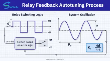
Relay autotuning, introduced by Åström and Hägglund in 1984, uses on-off control to generate sustained oscillations. The relay switches the control signal between two fixed levels based on the sign of the error, driving the system into a limit cycle.
By measuring the oscillation period and amplitude, the autotuner identifies the ultimate gain (Ku) and ultimate period (Pu). Ku is the proportional gain at which the closed-loop system becomes marginally stable; Pu is the resulting oscillation period.
Advantages: Relay methods are model-light, require no prior plant knowledge, and generate clear oscillatory data for frequency-domain identification.
Limitations: Deliberately creating oscillations can be unsafe in constrained or hazardous processes, and the method assumes the plant can tolerate sustained cycling.
Computing Gains from Plant Data
Once the autotuner estimates plant characteristics—whether frequency response, step features, or ultimate gain—it applies tuning formulas to calculate Kp, Ki, and Kd. The formulas target specific closed-loop properties:
- Phase margin: Typically 60° in documented implementations, providing robustness against modeling errors and parameter variations
- Gain margin: Adequate distance from instability
- Crossover frequency: Determines closed-loop bandwidth and response speed
The choice of formula depends on the autotuning method:
- Ziegler-Nichols produces aggressive, fast-responding controllers
- AMIGO prioritizes disturbance rejection with robustness constraints
- Model-based methods fit transfer functions and apply analytical design rules
- Optimization-based approaches minimize cost functions subject to stability constraints
Autotuning Methods and Algorithms
Ziegler-Nichols Methods
The foundational 1942 Ziegler-Nichols rules remain widely used because they are simple and need little plant modeling. Two variants exist:
Ultimate Cycle Method (Closed-Loop):
- Set integral and derivative gains to zero
- Increase proportional gain until sustained oscillation occurs
- Record the ultimate gain (Ku) and oscillation period (Pu)
- Apply the formulas:
- Kc = 0.6 Ku
- Ti = Pu / 2
- Td = Pu / 8
Reaction Curve Method (Open-Loop):
- Apply a step input and record the response
- Approximate the plant as first-order-plus-dead-time: Kproc (gain), L (delay), T (time constant)
- Calculate:
- Kc = 1.2T / (Kproc × L)
- Ti = 2L
- Td = 0.5L
Trade-off: Ziegler-Nichols rules produce aggressive controllers with fast response but limited robustness. They suit applications where speed matters more than smooth regulation, but often require detuning in practice.
AMIGO Tuning
AMIGO (Approximate M-constrained Integral Gain Optimization) was developed to improve disturbance rejection while maintaining robustness. It assumes an FOPDT plant model and optimizes integral gain subject to stability constraints.
AMIGO formulas:
- Kc = (0.2 + 0.45T/L) / Kproc
- Ti = L(0.4L + 0.8T) / (L + 0.1T)
- Td = 0.5LT / (0.3L + T)
AMIGO produces less aggressive controllers than Ziegler-Nichols, trading some speed for better margins and disturbance handling. It works well for monotone processes with moderate delays but still requires accurate FOPDT identification.
Model-Based Methods
When a single FOPDT formula is too coarse, model-based autotuning fits a parametric transfer function from step or frequency-response data. Common structures include FOPDT, second-order-plus-dead-time (SOPDT), or higher-order forms. Analytical tuning rules are then applied to the identified model.
The results stay interpretable: engineers can inspect the fitted model, check its accuracy, and see why specific gains were chosen.
Advantages:
- Handles delays explicitly
- Supports higher-order dynamics
- Enables "what-if" analysis by retuning the identified model with different criteria
Limitations:
- Accuracy depends on model fit
- Fast or oscillatory dynamics may require SOPDT or higher-order identification
- Poorly excited plants yield poor models
Optimization-Based Approaches
If fixed rules still fall short, optimization treats PID tuning as a constrained search: minimize a cost function (IAE, ISE, or ITAE) subject to stability and robustness limits.
Common cost functions:
- IAE (Integral Absolute Error), ∫|e(t)|dt, penalizes all errors equally
- ISE (Integral Squared Error), ∫e²(t)dt, penalizes large errors quadratically
- ITAE (Integral Time-weighted Absolute Error), ∫t|e(t)|dt, weighs errors more as time goes on
These criteria are distinct, not interchangeable. ITAE, for example, favors controllers that settle quickly, while ISE emphasizes minimizing large transient errors.
Trade-off: Optimization offers the most flexibility for multi-objective criteria. It also needs more computation, can settle in local minima, and gives less intuitive insight than formula-based methods.
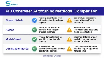
Method Comparison Summary
| Method | Strength | Limitation |
|---|---|---|
| Ziegler-Nichols | Simple, fast response | Aggressive, limited robustness |
| AMIGO | Better disturbance rejection, robustness constraints | Requires FOPDT approximation |
| Model-based | Handles delays, interpretable | Depends on model accuracy |
| Optimization | Flexible, multi-objective | Computationally intensive, less intuitive |
Applications and Use Cases
PID autotuning shows up wherever fixed gains struggle to keep up—industrial loops, motion systems, and certified vehicle or engine controls.
Industrial Process Control
Temperature, flow, and pressure regulation represent classic PID applications. Plant dynamics are typically slow (seconds to minutes), and autotuning can run safely during commissioning or scheduled maintenance windows. Step-response or relay methods work well, particularly for monotone, stable processes.
Example: In a 2025 photobioreactor pH trial, setpoint-relay autotuning ran for five days on a semi-industrial raceway reactor. It cut pH oscillation and rejected disturbances faster than classical relay tests while staying in closed-loop operation.
Motion Control
Servo systems and robotics demand fast response and tight tracking. Plant parameters change with load, inertia variations, and friction, making fixed-gain controllers suboptimal. Autotuning enables adaptive control: when the system detects parameter drift, it retunes online to restore performance.
Example: A 2014 PMSM motor study used relay autotuning for current and speed loops. It targeted a 60° phase margin and reached bandwidths of several hundred Hz (current) and tens of Hz (speed) without accurate motor parameters.
Aerospace and Automotive
Engine control and flight control systems operate under strict certification requirements and reliability standards. Manual tuning across the full operating envelope (altitude, Mach number, temperature, load) is prohibitively expensive. Autotuning reduces commissioning time, but every gain schedule must still pass pretest simulation and hardware-in-the-loop testing before certification. Teams usually lock candidate gains in simulation first, then confirm stability margins on the bench or HIL rig.
PID Autotuning in Gas Turbine Control Systems
Gas turbines present unique control challenges: nonlinear dynamics, multi-variable interactions (speed, temperature, pressure, surge margin), and wide operating-point variations (startup, idle, full power, transients). A single PID tuning rarely works across the entire envelope, so teams often rely on autotuning at key operating points and gain scheduling (adjusting parameters by condition) between them. Those scheduled or autotuned controllers still need validation before hardware testing.
Why Simulation Matters
Testing control laws directly on physical gas turbine hardware is expensive, time-consuming, and risky. Compressor stall, turbine overtemperature, or instability during transient maneuvers can damage engines or endanger test facilities. A 2005 Rolls-Royce Spey study used gain-scheduled PID controllers because engine response varied across the operating range. The team tuned controllers against ITAE objectives in simulation when physical engines were not available for implementation.
Similarly, NASA validated PI gain schedules for the STARC-ABL/NEAT propulsion system across altitude, Mach, and power operating points through pretest simulation followed by real-time hardware-in-the-loop tests. Measured results agreed with predictions, and degradation tests covering nominal, midlife, and end-of-life scenarios reported no compressor stalls.
SimTurbo: Physics-Based Control Validation
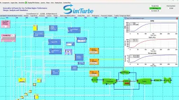
SimTurbo provides a gas turbine simulation platform for PID control development and validation before hardware implementation. The component-based environment includes drag-and-drop engine elements (inlets, compressors, combustors, turbines, nozzles, shafts) plus configurable PID controllers, limiters, actuators, sensors, and FADEC logic.
Key capabilities for PID tuning:
- Speed, temperature, and surge-margin PID blocks that drop directly into the engine model
- Live adjustment of PID settings while watching RPM, exhaust gas temperature (EGT), thrust, fuel consumption, and surge margin
- J85-GE-21 single-spool turbojet model validated against NASA Lewis Research Center test data, within ±2% on thrust, flow rate, temperature, and TSFC
- Startup, slam acceleration, throttle steps, stall/surge, sensor faults, and FADEC responses without risking hardware
- CSV or Excel export of RPM, EGT, thrust, and SFC for MATLAB, Python, or other post-processing
Engineers can autotune or hand-tune PID gains across the envelope, exercise gain schedules at off-design altitude, Mach, and temperature points, and check closed-loop behavior against physics-based plant dynamics before HIL or engine test. That pretest record is useful evidence when control laws move onto hardware.
Best Practices and Considerations
When to use autotuning
Autotuning helps most when dynamics are uncertain or have changed:
- Commission new systems when dynamics are known only approximately and you need efficient initial tuning
- Retune after hardware changes, retrofits, or process upgrades that invalidate existing gains
- Identify legacy or black-box plants that lack design records
- Recover when manual tuning leaves instability, weak disturbance rejection, or conflicting performance goals
When not to use autotuning
Not every system suits automated tuning. Screen out applications where safe, informative test signals cannot be guaranteed:
- Skip highly nonlinear plants: single-point gains hold only near the test operating point; wide ranges need scheduled tuning and envelope validation
- Avoid batch processes with cycle-to-cycle variation that block accurate identification
- Do not run tests on systems with hard constraints if signals could breach safety limits, damage equipment, or violate quality specs
Each application needs a safety analysis before you proceed—there is no blanket ban, only a duty to confirm the test is safe.
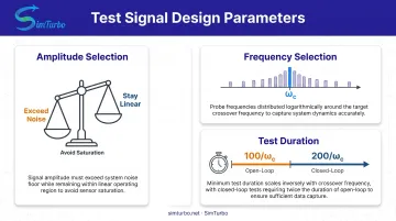
Test signal design recommendations
Amplitude selection:
- Large enough to exceed sensor noise and actuator deadband
- Small enough to remain within the locally linear region
- Avoid input saturation or output constraint violations
Frequency selection:
- Scale test frequencies to expected plant bandwidth
- Do not copy absolute Hz values from another application
- Probe frequencies around the target crossover frequency
Test duration:
- Continue until estimates stabilize
- Plan on about 100/ωc for open-loop tests and 200/ωc for closed-loop tests per MathWorks guidance
- Allow time for transient settling and noise averaging
Frequently Asked Questions
What is a PID autotune?
PID autotune is an automated procedure that calculates optimal controller gains (Kp, Ki, Kd) by testing the plant and analyzing its response. It replaces manual trial-and-error with controlled test signals and established tuning algorithms.
Can AI tune a PID loop?
Yes. AI and machine learning can tune PID controllers through reinforcement learning or historical data. Traditional methods such as Ziegler-Nichols remain more common in industry because of reliability, interpretability, and certification requirements.
How long does PID autotuning take?
Duration depends on plant dynamics and method. Fast servo systems may finish in seconds to minutes; slow thermal or chemical processes can take tens of minutes to hours. Relay tests need several oscillation cycles, while step-response methods need enough time for the plant to settle.
Is autotuning better than manual tuning?
Autotuning is faster and more consistent, especially when commissioning multiple systems or retuning after process changes. Skilled manual tuning can still win when constraints are unusual or dynamics don't match autotuner assumptions. Many engineers use autotune as a starting point, then fine-tune by hand.
Can autotuning handle multi-variable control systems?
Standard PID autotuning is single-input, single-output (SISO). Coupled multi-variable systems usually need sequential loop tuning, decoupling, or advanced methods such as model predictive control (MPC). Some platforms add multi-loop tuning with interaction analysis beyond classical PID algorithms.
What software tools support PID autotuning?
Siemens TIA Portal, Rockwell Automation, LabVIEW, and MATLAB/Simulink all include built-in PID autotuning tools. For gas turbine control, SimTurbo provides integrated PID components, real-time transient simulation, and validated engine models so you can develop and test control laws before hardware implementation.