PID Controller Explained

Introduction

PID controllers run most industrial automation—from manufacturing lines and aerospace flight control to marine propulsion, power generation, and chemical plants. A widely cited 2001 peer-reviewed study estimated that more than 90% of control loops use PID-family algorithms, and most of those are configured as PI (Proportional-Integral) controllers.

That prevalence comes from reliability: they hold precise, stable control whether you are regulating furnace temperature or managing jet-engine thrust. Poorly tuned loops still waste energy, wear actuators, and leave operators fighting oscillations.

This guide breaks down what PID controllers are, how each component (Proportional, Integral, Derivative) works in practice, proven tuning techniques, and where they are applied across industries.

Key Takeaways

• PID controllers automatically correct a process variable to hold a desired setpoint without manual intervention
• Three terms work together: P reacts to present error, I clears accumulated offset, D dampens future trends
• Over 90% of industrial control loops use PID for temperature, pressure, flow, speed, and position
• Manual tuning, Ziegler-Nichols, and auto-tuning give systematic ways to dial in performance
• Simple to implement without a full system model, and reliable for linear single-loop applications

What Is a PID Controller?

A PID controller is a feedback-based control loop mechanism that automatically calculates and applies corrections to keep a process variable at a desired setpoint. It maintains precise, stable control of dynamic systems—temperature, pressure, flow rate, motor speed, or fuel flow and shaft speed on a gas turbine—without constant human adjustment.

The acronym breaks down into three control actions:

• Proportional (P): Corrects based on how large the error is right now
• Integral (I): Removes steady-state offset from error that builds up over time
• Derivative (D): Damps overshoot by responding to how fast the error is changing

The Feedback Loop Concept

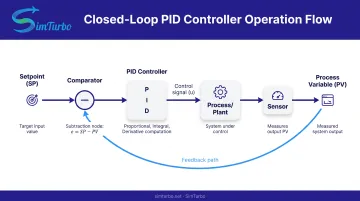
A PID controller operates in a closed loop by continuously measuring the difference between the setpoint (SP)—the desired value—and the process variable (PV)—the actual measured value. This difference is the error signal (e = SP - PV). The controller then adjusts the control output (also called the manipulated variable) to drive actuators like valves, motors, or heaters, working to minimize the error.

Closed-loop roles at a glance:

• Setpoint (SP): Target the loop is trying to hold
• Process variable (PV): Live measurement from sensors
• Error (e = SP − PV): Gap the controller works to drive toward zero
• Control output (u): Command sent to actuators (fuel valve, heater, motor drive)
• Sensors and actuators: Measure PV and apply the physical correction

Measure, compare, adjust—repeat. That cycle keeps the process on target as loads and operating conditions shift.

How Does a PID Controller Work?

A PID controller operates by combining three distinct control actions—proportional, integral, and derivative—each correcting error in a different way so the loop stays fast, stable, and accurate.

Proportional (P) Control

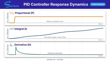
The proportional term produces an output directly proportional to the current error magnitude. Larger errors generate stronger corrective actions and a faster immediate response. If temperature is 10°C below setpoint, the heater increases power; if it is only 2°C below, the correction is gentler.

Proportional gain (Kp) sets how aggressively the controller responds. Higher gain increases responsiveness and shortens rise time, so the process variable reaches the setpoint faster. Excessive gain, however, causes overshoot (the process variable exceeds the setpoint) and oscillation (repeated cycling above and below the target).

Proportional control alone cannot eliminate steady-state error. The system settles close to the setpoint, but not exactly on it.

Integral (I) Control

The integral term accumulates error over time and increases correction based on how long the error persists. If temperature stays 1°C below setpoint for an extended period, the integral action builds up and applies additional corrective power until the offset disappears. This eliminates the steady-state error that proportional control alone cannot remove.

Integral gain (Ki) and integral time (Ti) control how quickly this correction grows. Faster integral action removes offset sooner, but too much aggressiveness can cause overshoot and oscillation.

A common challenge is integral windup. When an actuator hits a physical limit (a valve fully open, for example), the integral term keeps accumulating error even though the plant cannot respond further. When conditions change, that stored error drives excessive overshoot. Anti-windup methods pause or reset the integral term during saturation to prevent this.

Derivative (D) Control

The derivative term responds to the rate of change of error, providing anticipatory action that adds damping. If temperature is falling quickly toward the setpoint, derivative action cuts correction early and helps prevent overshoot. This improves settling time and reduces oscillations during rapid changes.

Derivative gain (Kd) and derivative time (Td) set the strength of this damping. Derivative action can improve stability and cut overshoot, but it is highly sensitive to measurement noise: small, rapid sensor fluctuations can trigger large, unnecessary corrections. For that reason, derivative action is often omitted or heavily filtered. Many industrial loops run as PI only.

Combined PID Action

The three terms work together through this combination:

u(t) = Kp × e(t) + Ki × ∫e(t)dt + Kd × de(t)/dt

Where:

• u(t) — control output
• e(t) — error at time t (setpoint − process variable)
• Kp, Ki, Kd — proportional, integral, and derivative gains

Proper tuning balances speed, stability, and accuracy. In a temperature loop, for example:

• P applies immediate heating in proportion to the current temperature error
• I removes lingering offset if the system settles 2°C below setpoint
• D eases heating as temperature nears a new setpoint, limiting overshoot

PID Controller Tuning

Tuning a PID controller means setting the Kp, Ki, and Kd gains so a specific system responds quickly, stays stable, and holds the setpoint. The usual targets are short rise time, limited overshoot, fast settling, and zero steady-state error.

Why Tuning Is Necessary

Every process has its own dynamics—time constants, delays, nonlinearities, and load disturbances—so default gains rarely work well. Response also differs by plant type:

• A furnace heating air reacts slowly to energy input
• A motor holding position responds much faster
• A valve regulating pressure sits somewhere in between

Without tuning matched to those dynamics, you get instability, large overshoot, or a sluggish loop that never quite settles.

Manual Tuning Approach

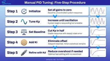
Manual tuning provides a systematic starting point:

1. Set Kp, Ki, and Kd to zero
2. Raise Kp until the loop oscillates at constant amplitude
3. Cut that Kp in half for a stable proportional baseline
4. Increase Ki until steady-state offset disappears
5. Add Kd only if overshoot or settling time still needs work

Effects of increasing each gain:

Gain	Rise Time	Overshoot	Settling Time	Steady-State Error
Kp	Decreases	Increases	Small change	Decreases (not to zero)
Ki	Decreases	Increases	Increases	Eliminates
Kd	Minor effect	Decreases	Decreases	No effect

These are tendencies, not absolute rules. Actual effects depend on system dynamics and require testing to confirm.

Ziegler-Nichols Method

The Ziegler-Nichols method is a classic tuning technique that determines PID parameters through systematic testing. The closed-loop approach works as follows:

1. Disable integral and derivative action (Ki = 0, Kd = 0)
2. Raise Kp until the loop holds a sustained, constant-amplitude oscillation
3. Record the ultimate gain (Ku) and oscillation period (Pu)
4. Compute Kp, Ki, and Kd from the standard Ku/Pu formulas

Ziegler-Nichols gives a clear starting point, but the resulting gains are often aggressive. Many loops still need manual refinement before they meet overshoot and robustness targets.

Modern Software-Based Tuning

Many PLCs (Programmable Logic Controllers) and DCS (Distributed Control Systems) now include auto-tuning features that automatically determine optimal gains through system identification. The controller perturbs the process with small test signals, observes the input/output response, and calculates appropriate PID parameters.

Simulation tools let you refine gains before you touch hardware. With SimTurbo, aerospace and marine engineers can run PID strategies for speed, temperature, and surge-margin control in real time, then stress them through startup and throttle transients.

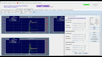
You can tweak Kp, Ki, and Kd on the model, compare responses, and export results to MATLAB/Simulink or Python for deeper analysis—without risking a physical engine test cell on the first pass.

Applications and Use Cases

Process Control Applications

PID controllers hold setpoints when loads and disturbances change. Common loops include:

• Temperature regulation: Ovens, reactors, heat exchangers, and furnaces hold tight thermal setpoints
• Pressure control: Vessels, pipelines, and compressors stay within safe, efficient ranges
• Flow control: Pumps and valves meter flow in chemical processing, water treatment, and fuel delivery
• Level control: Tanks hold liquid level in storage, mixing, and separation processes

Motion Control Applications

PID controllers track velocity and position commands in:

• Motor speed and position control: Robotics, CNC machines, and conveyors keep motion on target
• Servo systems in aerospace: Control surfaces and engine actuators follow pilot commands; NASA’s Ares I used PID to set thrust-vector gimbal angles for pitch and yaw
• Automotive cruise control: Throttle adjusts automatically to hold a set vehicle speed

Industry-Specific Examples

• HVAC systems: Building temperature and humidity loops that track comfort setpoints
• Power generation: Boiler firing, steam and gas turbine speed, and fuel-flow control
• Aerospace and marine propulsion: Thrust, engine performance, rudder, and propeller-speed control
• Chemical processing: pH and concentration control in continuous reactors and blending lines

Advantages and Limitations of PID Controllers

PID remains the default feedback choice in many plants and products for good reason. It is also easy to ask more of a single loop than classical PID can deliver.

Key Advantages

• Simple to implement: Engineers can get effective results without deep control-theory background.
• No full plant model required: Empirical tuning and plant tests often beat building a detailed mathematical model first.
• Long track record: Ziegler-Nichols methods date to 1942, and later reviews still call PID the first feedback tool to try.
• Strong on linear single loops: Works well when dynamics stay relatively predictable across the operating range.
• Clear tuning playbooks: Manual tuning, Ziegler-Nichols, and auto-tuning give repeatable starting points.

Primary Limitations

• Deadtime hurts performance: Large transport or communication delays degrade classical PID, especially when delay exceeds the dominant time constant.
• Nonlinear plants drift off tune: One gain set can work at one operating point and fail at another, so gain scheduling is often required.
• Derivative noise sensitivity: D action amplifies measurement noise; heavy filtering or dropping D is common.
• Integral windup: When actuators saturate, the integrator keeps accumulating error and can drive large overshoot once the limit clears.

When PID May Not Be Sufficient

Advanced methods (model predictive control, adaptive control, or state-space techniques) may be needed for:

• Multivariable processes with strong loop interactions
• Constrained systems that must optimize inside operating limits
• Highly nonlinear dynamics that one PID gain set cannot cover
• Deadtime-dominant processes where delayed feedback caps achievable performance

Conclusion

PID controllers remain the workhorse of industrial control. They are simple to implement, effective across a wide range of plants, and flexible enough for everything from basic temperature loops to aerospace systems.

Know how the P, I, and D terms act on their own and together, and learn solid tuning habits. That foundation is what lets you keep loops stable and accurate when conditions change. The same structure shows up whether you are holding reactor temperature, trimming motor speed on an assembly line, or managing thrust on a gas turbine—and in simulation tools used to design those turbine controls before hardware testing.

Frequently Asked Questions

What does PID control mean?

PID stands for Proportional-Integral-Derivative control. It calculates the error between a desired setpoint and the actual process variable, then applies three corrective actions to reduce that error and keep the process stable.

What is a PID controller example?

Cruise control is a common example: the PID controller holds a set speed by adjusting throttle. When the car hits a hill and slows, it increases throttle to restore the target speed without driver input.

How do you tune a PID controller?

Tuning means adjusting three gain parameters (Kp, Ki, Kd) to balance response speed, stability, and accuracy. Common methods include manual tuning (adjust gains while watching the response) and auto-tuning routines such as Ziegler-Nichols.

What is the difference between P, PI, and PID controllers?

A P controller uses only proportional action and leaves steady-state error. PI adds integral action to eliminate offset and is the most common industrial choice. PID adds derivative action when you need faster response with less overshoot.

What are the main advantages of PID controllers?

PID controllers are simple to implement, need no detailed process model, and work across many applications. With well-established tuning methods and reliable performance, they remain the industry standard for most control loops.

Where are PID controllers most commonly used?

They are widely used in process industries (temperature, pressure, flow, level), manufacturing automation, HVAC, aerospace and marine propulsion, chemical processing, and power generation. In short, any application that needs automatic regulation of a process variable.