PID Controller Design

Many engineers face a recurring challenge: how to maintain stable, accurate control in systems where operating conditions change constantly. A temperature controller that works perfectly at low loads may oscillate wildly under peak demand. A motor speed regulator tuned for one setpoint overshoots dramatically when asked to track a different target. According to ISA, PID controllers remain the most common industrial closed-loop technology, and a 2016 industry study found that 97% of regulatory controllers still rely on PID feedback algorithms. This article explains how PID controllers work, how to tune them effectively, and how modern simulation platforms like SimTurbo enable engineers to validate control strategies before deploying them on physical systems.

Key Takeaways:

• PID controllers combine proportional, integral, and derivative actions to eliminate error and improve stability
• Proper tuning balances response speed against overshoot and oscillation
• Most industrial loops use only P or PI control; full PID is reserved for specific damping needs
• Modern simulation tools allow safe testing of control strategies before real-world deployment

How PID Controllers Work

A PID controller continuously measures the difference between a desired setpoint and the actual process variable, called the error signal, and calculates a corrective output to drive that error toward zero. The feedback loop operates in four steps:

1. Measure the process variable (temperature, speed, pressure, etc.)
2. Calculate error as e = setpoint – measured value
3. Compute control output using proportional, integral, and derivative terms
4. Apply correction to the actuator (valve, motor, heater, etc.)

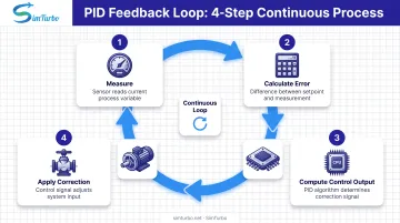
This cycle repeats continuously while the controller is active.

Cruise Control as a Feedback Example

Consider automotive cruise control. You set a target speed of 65 mph (setpoint). The system measures your current speed via a sensor (process variable). If you're traveling at 60 mph, the error is +5 mph, and the controller increases throttle in proportion to that error.

As speed approaches 65 mph, the error shrinks and throttle adjustment becomes gentler. If a hill slows you to 63 mph, the controller detects the new error and adds more throttle until you return to setpoint.

Cruise control makes the feedback loop concrete: measure, compute error, correct—and keep doing it so the process holds the target under changing load.

Understanding the Three PID Components

Each PID term corrects error in a different way. Proportional reacts to present error, integral clears accumulated offset, and derivative damps rapid change.

Proportional (P) Control

Proportional control generates an output directly proportional to the current error, scaled by a gain constant Kp. If error doubles, output doubles.

Key effects of increasing Kp:

• Faster initial response and shorter rise time
• Reduced steady-state error
• Increased risk of oscillation and overshoot

Critical limitation: P-only control cannot eliminate steady-state error completely. It requires a non-zero error to produce output, so the system settles at a small offset from the setpoint. ISA notes that proportional action alone leaves an offset that must be corrected by integral action.

Integral (I) Control

Integral control sums error over time, continuously accumulating the correction needed. This eliminates steady-state error because even a tiny persistent offset will eventually build enough integral action to drive it to zero.

Key effects of increasing Ki:

• Eliminates steady-state error completely
• Faster removal of residual error
• Increased overshoot and potential oscillation if set too high

Integral windup occurs when the actuator saturates (reaches its physical limit) but the integral term keeps accumulating error. When the actuator finally unsaturates, that built-up integral can cause large overshoot.

MathWorks describes two common anti-windup strategies:

• Clamping: Stops integration while the actuator is saturated
• Back-calculation: Feeds the saturation error back to unwind the integrator

Derivative (D) Control

Derivative control responds to the rate of change of error, providing anticipatory action that improves stability. It acts like a brake, slowing the approach to setpoint and reducing overshoot.

Key effects of increasing Kd:

• Reduced overshoot
• Improved damping and stability
• Faster settling time
• High sensitivity to measurement noise

Why derivative is used sparingly: Measurement noise (small rapid fluctuations in sensor readings) creates large derivative spikes. Those spikes amplify control output swings, wear actuators, and degrade performance.

An IFAC study recommends designing measurement filters jointly with PID tuning rather than relying on defaults. In practice, many successful loops use only P or PI, reserving full PID for cases where damping benefits clearly outweigh noise sensitivity.

PID Tuning Methods

Choosing optimal PID gains requires balancing competing goals: fast response, minimal overshoot, zero steady-state error, and stable behavior under disturbances.

Manual Tuning Approach

ISA recommends a conservative, step-by-step manual procedure:

1. Set Ki = 0 and Kd = 0
2. Increase Kp until the system oscillates with constant amplitude
3. Reduce Kp by 30-50% to restore stability with acceptable error
4. Add small Ki to eliminate steady-state error; watch for overshoot
5. Add Kd only if damping is needed and noise permits

Effect of Increasing Each Parameter:

Parameter	Rise Time	Overshoot	Settling Time	Steady-State Error	Stability
Kp	Decrease	Increase	Small change	Decrease	Degrade
Ki	Decrease	Increase	Increase	Eliminate	Degrade
Kd	Minor change	Decrease	Decrease	No effect	Improve if not noisy

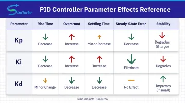
University of Michigan cautions that these effects are typical but not universal; actual plant dynamics determine the true response.

Ziegler-Nichols Method

The Ziegler-Nichols closed-loop method offers an empirical starting point. The classical four-step procedure is:

1. Set integral time to maximum and derivative to zero
2. Increase proportional gain until the system oscillates with constant amplitude
3. Record the ultimate gain Ku and oscillation period Pu
4. Calculate PID gains using standard formulas

Standard Ziegler-Nichols gain formulas:

• P controller: Kp = 0.5 Ku
• PI controller: Kp = 0.45 Ku, Ti = Pu / 1.2
• PID controller: Kp = 0.6 Ku, Ti = Pu / 2, Td = Pu / 8

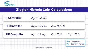
Trade-offs: The method requires no mathematical model and works across many systems, but it deliberately pushes the plant to instability during testing, which is unsafe for critical processes. The resulting gains can be aggressive, so most plants need further refinement.

Modern Software-Based Tuning

Modern tuning software uses system identification and optimization algorithms to calculate PID parameters automatically.

Relay auto-tuning induces a controlled limit cycle with a relay switch, then estimates plant gain and frequency from the oscillation amplitude and period. This avoids the instability risk of direct ultimate-gain testing, though reported ultimate-gain errors can reach 5-20%.

Model-based approaches fit plant dynamics to first-order-plus-delay or higher-order transfer functions. Rules such as AMIGO (Approximate M-constraint Integral Gain Optimization) then balance performance and robustness.

Simulation-based tools let engineers test gain changes virtually, watch transient behavior, and validate control strategies before hardware deployment. That workflow cuts costly trial-and-error on physical systems. SimTurbo supports the same loop with built-in PID components and real-time transient engine simulation, so gains can be proven against a plant model first.

Common PID Design Challenges

Nonlinear Systems and Gain Scheduling

PID controllers are designed for linear systems where fixed gains work across all operating conditions. Real systems often behave nonlinearly: heat transfer rates change with temperature, aerodynamic forces vary with speed, and valve characteristics curve at extreme positions.

A peer-reviewed aircraft engine study documents gain-scheduled PID for gas turbines because engine dynamics shift dramatically across the flight envelope.

Single fixed gains cannot deliver acceptable performance at idle, cruise, and maximum thrust at once. Gain scheduling switches PID parameters by operating point, at the cost of higher design complexity and a heavier validation burden.

Deadtime and Time Delay

Deadtime, the delay between a control action and its measurable effect, degrades PID performance and erodes stability margins. Long delays keep the controller from reacting promptly to disturbances, so the loop can overcorrect once feedback finally arrives.

For delay-dominated processes, PI control often outperforms full PID because derivative action offers minimal benefit when feedback is already stale.

Measurement Noise Amplification

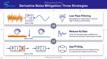
Derivative control calculates the rate of change of error. Small high-frequency noise in the sensor signal creates large derivative spikes that cause unnecessary actuator movement, mechanical wear, and reduced control quality.

Common mitigation strategies:

• Apply low-pass filtering to the measurement signal before derivative calculation
• Reduce Kd to limit derivative contribution
• Omit derivative entirely and use PI control

An IFAC paper stresses that measurement-filter design should be part of PID tuning, not an afterthought.

PID Controller Applications Across Industries

Process and Manufacturing Control

Chemical Temperature Control: A 2023 cascade-control case study describes PID regulation of reactor temperature through a slave loop controlling jacket heat-transfer-fluid temperature and split-range hot/cold valves. The master PID stabilizes reactor temperature while the slave loop handles faster thermal dynamics.

Motor Speed Control: A 2022 IFAC paper addresses DC motor speed regulation under linear and nonlinear mechanical loads using PID control. The controller maintains constant speed despite load variations by adjusting motor voltage based on measured speed error.

Hydraulic Pressure Regulation: Fluid-power systems use PID for cylinder position, hydraulic-motor speed, and pressure control. Derivative action remains susceptible to sensor and discretization noise in these high-bandwidth applications.

Gas Turbine Engine Control

Gas turbine engines present demanding control challenges: highly nonlinear dynamics, wide operating ranges, stringent safety limits, and fast transient requirements. NASA documentation explains that fuel schedules meter combustor fuel flow while maintaining maximum/minimum limits to protect against surge, over-temperature, overspeed, and flameout.

PID controllers regulate:

• Fuel flow to maintain desired thrust or speed
• Turbine inlet temperature to prevent material damage
• Compressor surge margin to avoid aerodynamic instability
• Engine speed during acceleration and deceleration

The 2005 aircraft engine study used gain-scheduled PID tuned by ITAE (Integral Time Absolute Error) optimization because fixed gains cannot accommodate the nonlinear behavior across idle, cruise, and maximum thrust.

Real-Time Control Validation in SimTurbo

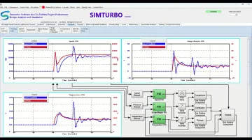
Before hardware runs, engineers validate PID loops against physics-based engine models. SimTurbo, from Controls Research LLC, is a component-based gas turbine simulation environment for building those closed-loop systems from graphical blocks.

Engineers wire PID controllers, limiters, actuators, sensors, compressors, combustors, turbines, and nozzles, then configure speed, temperature, and surge-margin PIDs. Real-time graphs compare setpoints with sensor feedback during events such as:

• Startup sequences
• Throttle changes and slam accelerations
• Sensor-failure scenarios

SimTurbo's J85-GE-21 validation case matched thrust, flow rate, temperature, and TSFC predictions within ±2% of NASA test data. Engineers can export transient results to CSV or Excel for post-processing in MATLAB, Simulink, or Python, then refine tuning before deploying on a physical engine.

Best Practices for PID Implementation

Choose the Simplest Effective Controller Structure

Not every application needs full PID. ISA recommends using only the control terms your requirements demand:

• P control: Acceptable when small steady-state error is tolerable
• PI control: Use when zero steady-state error is required and derivative noise is problematic
• PID control: Use when you need fast response and low overshoot, and derivative benefit outweighs noise risk

Many successful industrial loops use only P or PI because derivative action adds complexity, noise sensitivity, and often marginal performance gain.

Prioritize Sensor Selection and Measurement Quality

PID performance depends directly on accurate, timely process measurements. Poor sensor selection undermines even perfectly tuned controllers.

Sensor requirements:

• Range and accuracy matched to process variable and control tolerance
• Bandwidth sufficient to capture process dynamics
• Resolution fine enough to detect meaningful changes
• Low noise or effective filtering

Match sampling rate to plant dynamics. A 2016 peer-reviewed study found that larger sample periods worsen control quality and can destabilize some discretizations.

As a rough guideline, sample 10–20× faster than the system’s natural response time. Then validate digital implementations against their continuous-time counterparts.

Implement Anti-Windup Protection

Actuator saturation is inevitable: valves hit fully open or closed, motors reach speed limits, and heaters hit maximum output. Without anti-windup protection, the integral term keeps accumulating error during saturation and drives large overshoot when the actuator unsaturates.

Anti-windup strategies:

• Clamping (conditional integration): Stop integration when output saturates
• Back-calculation: Feed the difference between saturated and unsaturated output back to unwind the integrator
• Integral limits: Cap the maximum integral value

Test recovery behavior after sustained saturation to ensure smooth return to normal operation.

Start Conservative and Tune Iteratively

When instability can damage equipment or create safety hazards, start with lower gains and raise them iteratively.

Safe commissioning sequence:

1. Start from a known stable baseline
2. Excite the system within safe limits
3. Change one parameter at a time
4. Observe response to setpoint changes, disturbances, and operating-point shifts
5. Retest across the full operating envelope

Conservative tuning rules trade some performance for greater stability margins. The AMIGO method exemplifies this philosophy, prioritizing robustness over aggressive response.

Frequently Asked Questions

What is the difference between P, PI, and PID controllers, and when should I use each?

P control reacts only to present error and leaves steady-state offset. PI adds integral action to remove that offset but can increase overshoot. PID adds derivative damping to cut overshoot and speed settling; use the simplest structure that meets your specs (many industrial loops need only PI).

How do I know if my PID controller is properly tuned?

A well-tuned controller reaches setpoint quickly without excessive overshoot, exhibits minimal oscillation, and settles within acceptable time for your application. Performance criteria are plant-specific; there is no universal overshoot or settling target. Monitor disturbance rejection and actuator activity as well.

Why does my PID controller oscillate or become unstable?

Oscillation typically results from excessive loop gain (especially Kp or Kd) or inadequate damping. Reduce gains systematically, check for measurement noise, verify sampling rate is adequate, and confirm the plant hasn't changed operating conditions. Unwanted cycling differs from ultimate-sensitivity oscillation used on purpose in Ziegler-Nichols tuning.

What causes integral windup and how can I prevent it?

Windup occurs when the actuator saturates but integration continues accumulating error. Prevent it by clamping the integral term during saturation, using back-calculation to unwind it, or temporarily disabling integration. Test recovery behavior after sustained saturation events.

Can PID controllers work with nonlinear systems?

PID works well with mildly nonlinear systems over a validated operating range. When dynamics change sharply with operating point, you need gain scheduling, adaptive control, or model-based methods. The aircraft gas turbine study used gain-scheduled PID because one fixed gain set could not cover the full flight envelope.

What sampling rate do I need for digital PID implementation?

Sampling should be fast enough to capture process dynamics accurately and avoid aliasing. A common rule of thumb is 10-20× faster than the system's natural response time, though sample-period guidelines are only rough estimates and discrete PID still needs sample-aware retuning. Validate your digital implementation against the continuous design.