Introduction
Engineers designing and operating gas turbine engines, whether for aerospace, marine propulsion, or power generation, face a fundamental choice: steady state or transient modeling. Each approach serves distinct analysis goals, and selecting the wrong one wastes time and resources.
According to NASA, increasing development costs and operational risks have intensified the industry's dependence on mathematical models for gas turbine design.
Steady state analysis captures equilibrium performance at fixed design points such as cruise altitude or constant load. Transient modeling tracks time-dependent behavior during startup, throttle changes, and control-system response.
This article explains what steady state modeling is, how it differs mathematically and computationally from transient simulation, and when each approach fits. You will get the core math, practical turbine applications, validation benchmarks, and practices that keep results accurate.
Key Takeaways
- Steady state models set time derivatives to zero and solve algebraic equations for design-point equilibrium
- Transient runs integrate differential equations over time for startup, control checks, and dynamic response
- NASA T-MATS treats steady state as unchanging with time; dynamic sims support controls work
- SimTurbo steady-state results match NASA test data within ±2% on thrust, flow rate, and fuel burn
- Component-based setups map performance and efficiency without treating the engine as a black box
What is Steady State Modelling?
What is Steady State Modeling?
Steady state modeling captures the equilibrium condition of a gas turbine system where key variables (pressure, temperature, mass flow rates, and shaft speed) remain constant over time. NASA defines a steady-state simulation as unchanging with time, distinguishing it from dynamic simulation that changes with time.
Steady state does not mean motionless. The compressor blades spin, air flows through the engine, and fuel burns continuously. Instead, it means that performance parameters have stabilized: thrust holds steady, exhaust gas temperature stops climbing, and rotor speed remains constant. At this equilibrium, mass flow entering each component equals mass flow leaving, and shaft torques balance.
Design Point vs. Transient Behavior
Steady state analysis focuses on long-term operating behavior at specific design points:
- A jet engine cruising at 35,000 feet with constant throttle
- A power generation turbine delivering steady electrical load
- A marine turbine maintaining a fixed vessel speed
By contrast, steady state modeling ignores transient effects such as:
- Engine startup sequences
- Throttle changes and acceleration
- Shutdown procedures
- Compressor surge events
- Control system responses to disturbances
Practical Examples
Aerospace: During takeoff, thrust ramps quickly and the engine runs transiently. Once the aircraft levels at cruise with fixed throttle, the same turbofan settles into steady state.
Power Generation: An aero-derivative turbine on baseload runs at steady state. When grid demand spikes and the unit answers a frequency-response event, it operates transiently.
This distinction determines which modeling approach delivers useful results. Design-point calculations, efficiency studies, and component sizing rely on steady state. Startup validation, control tuning, and fault-response prediction require transient analysis.
Steady State vs. Transient (Dynamic) Simulation
Fundamental Differences
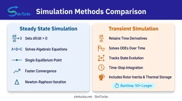
Transient simulation tracks how system variables evolve from one state to another, including the time-dependent path between equilibrium points. Steady state models reduce to algebraic component balances and matching residuals. Transient models keep ordinary differential equations (ODEs) with initial and boundary conditions for density, energy, and shaft speed.
Mathematical Approach:
- Steady state: Sets all time derivatives to zero (dX/dt = 0), converting differential equations into algebraic equations. Zero net shaft torque and component flow-matching become residuals to solve simultaneously.
- Transient: Retains time derivatives for rotor inertia, intercomponent volume filling, and thermal storage. NASA uses dN/dt = (Trq_comp + Trq_turb + Trq_other)/(2πI) to model shaft acceleration.
Computational Requirements:
Steady state simulations solve one converged operating point per condition using iterative methods like Newton-Raphson. Transient models require time integration plus repeated component matching at successive time steps.
Runtime ratios vary by model complexity and hardware. NASA reports that T-MATS generally executed faster than real time. One 2024 review found an intercomponent-volume transient method required 8 minutes versus 5 seconds for an alternate formulation. That comparison is between two transient approaches, not steady state versus transient.
When to Use Steady State Modeling
Steady state analysis excels for:
Design Point Analysis:
- Sizing compressors, turbines, and combustors at rated conditions
- Calculating thrust, power, and efficiency at specified operating points
- Creating performance maps across altitude, speed, and power settings
Initial Design Phases:
- Component matching to ensure compressor and turbine operating points align
- Pressure-ratio optimization
- Understanding equilibrium behavior before investing in detailed transient models
Certification & Compliance:
- FAA 14 CFR 33.85 requires calibration tests that establish power characteristics at stabilized conditions
- Demonstrating that steady operating points meet contractual specifications
- Generating compliance documentation for regulatory submissions
Efficiency & Fuel Consumption Studies:
- Evaluating specific fuel consumption (SFC) and thermal efficiency
- Meeting emissions and fuel-efficiency regulatory requirements
- Benchmarking performance against industry standards
When to Use Transient (Dynamic) Modeling
Transient analysis is essential when time-dependent effects matter:
Startup & Shutdown:
- Engine light-off sequences
- Acceleration from idle to full power
- Controlled shutdown procedures
Control System Validation:
- Tuning PID controllers and limiters
- Testing actuator response and sensor feedback
- Validating FADEC logic under dynamic conditions
Fault & Safety Analysis:
- Compressor surge detection and recovery
- Sensor failure response
- Emergency shutdown sequences
Hardware-in-the-Loop Testing:
- Real-time control validation
- Integration with physical controllers
- Rotor dynamics and thermal stress studies where time-history matters
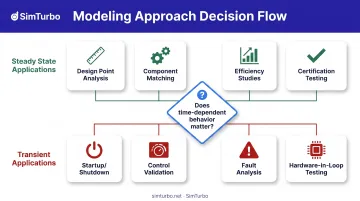
Choosing the right mode depends on whether you need equilibrium answers or time-history behavior. SimTurbo supports both steady state and transient analysis in one platform, so teams can move from design-point work to dynamic control validation without switching tools.
Mathematical Foundations of Steady State Analysis
At steady state, all time derivatives vanish. The governing equations simplify from differential to algebraic form, making numerical solution faster.
Setting Time Derivatives to Zero
NASA defines steady operation through dX/dt = 0, meaning no accumulation of mass, energy, or momentum within components. For shaft dynamics:
Transient: dN/dt = (Trq_comp + Trq_turb + Trq_other)/(2πI)
Steady State: 0 = Trq_comp + Trq_turb + Trq_other → net torque balances
Mass and Energy Conservation at Equilibrium
Mass Balance: Inlet flow equals outlet flow for each component. For a burner, W_out = W_in + W_f, where W_f is fuel flow.
Energy Balance: NASA's burner energy equation becomes ht_out = (W_in × ht_in + W_f × LHV × Eff)/W_out, where LHV is lower heating value and Eff is combustion efficiency. Pressure loss is modeled as Pt_out = (1 - dP) × Pt_in.
Component Matching Example: Compressor at Steady State
For a compressor at steady state:
- Flow Balance: Inlet mass flow = outlet mass flow (no accumulation)
- Energy Balance: Shaft power input = aerodynamic work on the air
- Map Matching: Thermodynamic corrected flow must match the compressor map at the current corrected speed and pressure ratio
Isentropic Relations: For ideal-gas assumptions, Tf/Ti = (Pf/Pi)^((γ-1)/γ), linking temperature ratio to pressure ratio through the specific heat ratio γ.
Solver Methodology
T-MATS uses Newton-Raphson iteration to converge the system of algebraic equations. Perturbing inputs builds the Jacobian, which is only locally valid for nonlinear systems, so convergence depends on initial guesses, perturbation sizes, and tolerances.
Eliminating time derivatives is why steady-state models run orders of magnitude faster than transient simulations. The limit is equally clear: steady state cannot show how the system moves between equilibrium points.

Applications of Steady State Modeling in Gas Turbine Engineering
Performance Analysis and Design Point Calculations
Engineers use steady state models to calculate thrust, power output, fuel consumption, and efficiency at specified operating conditions. NASA's gas turbine performance modeling techniques focus on design-point analysis to size or match components at specified mission points.
Performance Maps: Steady state analysis creates performance maps showing engine behavior across:
- Different altitudes and ambient temperatures
- Varying flight speeds or stationary load conditions
- Multiple power settings from idle to maximum thrust
SimTurbo's component-based architecture enables engineers to rapidly prototype configurations, run design-point calculations, and visualize results through real-time Temperature-Entropy (T-S) and Pressure-Volume (P-V) diagrams.
Performance curves can span corrected engine speeds from 4,000 to 20,000 RPM, displaying thermal efficiency (approximately 0.1–0.5) and thrust-specific fuel consumption (roughly 0.48–2.40 lb/hp/hr).
Validation Benchmark: NASA's J85-GE-21 validation case set reference design values of 2,850 lbf thrust, 0.99 SFC, 16,540 rpm, 44 lb/s flow, a compressor pressure ratio of 7, and a turbine-inlet temperature of 2,100°R.
Model results reached 2,861 lbf thrust (0.3% error), 0.9901 SFC (0.01% error), and 2,097°R (0.14% error). SimTurbo's J85-GE-21 validation achieved ±2% accuracy for thrust, flow rate, temperature, and TSFC against NASA test data.
Component Sizing and Matching
Steady state simulation helps engineers properly size compressors, turbines, combustors, and nozzles, then verify that their operating points are compatible at equilibrium.
Component Matching Process: Each turbomachinery component operates along characteristic curves (compressor maps and turbine maps). At steady state:
- Compressor corrected flow must match turbine corrected flow through continuity
- Compressor calculated corrected flow must equal the flow permitted by the map at corrected speed and operating line
- Shaft torques from all components must sum to zero
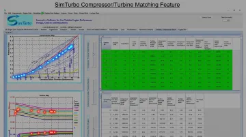
Identifying Mismatches: SimTurbo displays compressor and turbine maps with operating points plotted in real time. Engineers can:
- Detect when a compressor operates too close to surge line (low surge margin)
- Identify turbine choking that limits airflow
- Spot mismatches between compressor pressure ratio and turbine expansion ratio
- Adjust component sizes, speeds, or geometries before hardware commitment
These insights prevent performance shortfalls and mechanical failures that would be expensive to correct after manufacturing.
Efficiency and Fuel Consumption Studies
Steady state models calculate specific fuel consumption (SFC) and thermal efficiency at various operating points. Those results feed regulatory compliance work and cost optimization.
Current Industry Benchmarks:
| Engine Class | Power Output | Thermal Efficiency | Source |
|---|---|---|---|
| GE Vernova LM6000 PF+ Sprint | 56.9 MW | 41.0% (8,328 Btu/kWh) | ISO conditions, natural gas |
| Baker Hughes LM9000 (mechanical drive) | 73.1 MW | 44.2% | ISO, sea level, 60% RH |
| Baker Hughes LM9000 (power gen) | 70.2–71.4 MWe | 42.8–43.1% | ISO, natural gas, no losses |
Aerospace Fuel Consumption: NASA defines thrust-specific fuel consumption (TSFC) as TSFC = mdot_f/F, with typical sea-level-static teaching values of 1.0 lbm/(h·lbf) for turbojets and 0.5 lbm/(h·lbf) for turbofans. TSFC varies significantly with speed and altitude, so these are reference values, not universal cruise benchmarks.
Steady state efficiency and SFC work relies on thermodynamic cycle modeling, component performance maps, and operating-point analysis. Engineers evaluate fuel consumption, pressure-ratio effects, and off-design performance under different altitude and ambient conditions, then benchmark results against NASA engine testing.
Control System Design Validation
Steady state analysis establishes baseline operating points that control systems must maintain or transition between.
Baseline Operating Points: Before designing controllers, engineers need:
- Nominal thrust or power at cruise
- Temperature and pressure limits at maximum continuous power
- Idle fuel flow and rotor speeds
- Safe operating margins (distance from surge line, maximum turbine temperature)
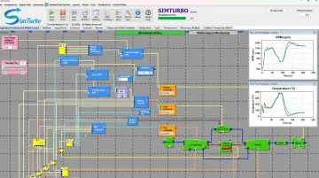
Control Set Points & Operating Limits: SimTurbo integrates PID controllers, limiters, actuators, and sensors with steady state engine models. Engineers can:
- Define RPM and temperature set points visible against real-time sensor feedback
- Monitor surge margin, often 20–25% during normal operation
- Configure Speed PID and Surge Margin PID control blocks
- Model fuel-flow modulation, nozzle-area changes, and variable stator-vane control
These steady state results initialize transient control validation, where engineers test PID tuning, limiter thresholds, and FADEC logic during dynamic maneuvers.
Certification and Compliance Testing
Aerospace and power generation industries require demonstration of steady state performance at specified conditions.
Regulatory Requirements:
- FAA 14 CFR 33.85 mandates calibration tests that establish turbine-engine power characteristics across speeds, pressures, temperatures, and altitudes, with each condition stabilized before measurement
- FAA 14 CFR 33.87 prescribes endurance schedules including repeated rated takeoff, maximum-continuous, idle, and cruise blocks
- EASA CS-E 730 requires pre/post-endurance calibration to identify thrust or power changes and confirm performance targets
Validation Process: Engineers compare simulation results against test data to demonstrate compliance. NASA T-MATS steady-state comparisons with NPSS showed all differences below 0.5%, including 0.15% for thrust. SimTurbo's J85-GE-21 validation within ±2% shows the accuracy steady state platforms can deliver for compliance documentation and regulatory submissions.
While regulations do not prescribe steady state simulation as the sole compliance method, validated models provide evidence that designs meet contractual performance specifications before expensive physical testing.
Tools and Best Practices for Steady State Simulation
Simulation Platform Selection
Choosing the right steady-state platform accelerates design cycles and improves result quality. Key features include:
Component-Based Architecture: Platforms like SimTurbo provide pre-built gas turbine components (compressors, combustors, turbines, nozzles, shafts, recuperators, afterburners) that users assemble graphically rather than coding from scratch. This approach:
- Exposes mass-flow relationships and pressure losses that black-box models conceal
- Enables rapid architecture changes (adding intercoolers, regenerators, or variable geometry)
- Supports drag-and-drop model assembly with real-time updates
Validated Physics Models: Prioritize platforms that ship:
- Industry-standard thermodynamic relations and gas-property tables
- Real-gas effects, not just ideal-gas assumptions
- Component maps calibrated at known design points, then applied off-design
- Documented validation against test data or reference codes
User-Friendly Interface: A strong interface should offer:
- Real-time performance graphs and thermodynamic cycle diagrams
- Interactive compressor and turbine maps with operating points plotted
- Windows-based GUI for design and analysis workflows
Platform Examples:
| Platform | Capabilities |
|---|---|
| NASA T-MATS | Steady-state and dynamic models; generic thermodynamic/control libraries; 0-D component models; iterative solver |
| NPSS | Preliminary design, off-design, transient performance, flight-test correlation modes; nonlinear thermodynamic environment |
| NASA pyCycle | Implicit residual-based cycle models with analytic derivatives for gradient optimization; matched NPSS within 0.03% |
| SimTurbo | Component-based Windows GUI; steady-state Brayton-cycle analysis and transient simulation; validated J85-GE-21 model within ±2%; supports PID, limiters, sensors |
Best Practices for Accurate Results
Platform choice sets the ceiling on accuracy; disciplined setup determines whether you reach it.
Start with Validated Component Models: Calibrate compressor and turbine map scalars at a known steady design point, then apply them off design. Generic maps may match near design but diverge materially away from it.
Specify Proper Initial Conditions & Boundary Conditions: Poor initial guesses can prevent Newton-Raphson solvers from converging. Start with:
- Reasonable estimates for pressures, temperatures, and flows
- Shaft speeds near expected operating points
- Component efficiencies consistent with the design class
Conduct Sensitivity Analysis: Test how key parameters and numerical settings affect results:
- Vary compressor efficiency ±2% and observe thrust/SFC changes
- Adjust turbine-inlet temperature and check margin to material limits
- pyCycle showed derivative error reaching 100% when finite-difference steps fell below a solver tolerance, demonstrating that tolerance settings matter
Document Convergence Variables: Track residual definitions, initial guesses, Jacobian perturbations, tolerances, iteration limits, and restart policy. This documentation enables troubleshooting and ensures repeatability.
Validate Hierarchically:
- Component equations/maps → independent cycle code → measured engine data
- NASA examples used both NPSS cross-comparison and experimental/engine-reference data
- SimTurbo's J85-GE-21 validation against NASA test data provides confidence in steady-state accuracy
Integration with Design Workflow
Once steady-state models are trustworthy, fold the outputs into the rest of the design process.
Feed Downstream Analysis: Steady-state results inform:
- Structural analysis (blade stresses at rated conditions)
- Thermal analysis (heat-transfer loads and material temperatures)
- Dynamic analysis (initialization for transient startup/shutdown studies)
Export for Post-Processing: SimTurbo and similar platforms export steady-state data to MATLAB, Excel, or Python, enabling:
- Custom performance plots and trade studies
- Optimization loops that iterate design variables
- Integration with broader system models (aircraft performance, power-plant economics)
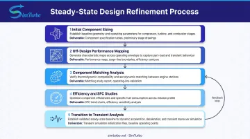
Iterative Design Refinement: Use steady-state analysis early and often:
- Initial component sizing at design point
- Off-design performance mapping to verify operating envelope
- Component matching to identify incompatibilities
- Efficiency and SFC studies to meet targets
- Transition to transient analysis only after steady-state design is mature
This workflow minimizes computational cost and focuses expensive transient simulations on validated designs.
Frequently Asked Questions
What are steady-state models?
Steady-state models are mathematical representations of gas turbine systems at equilibrium, where pressures, temperatures, flow rates, and shaft speeds remain constant over time. NASA defines them as unchanging with time, solving algebraic equations with time derivatives set to zero.
What is the difference between steady-state and transient state analysis?
Steady-state analysis solves algebraic equations at a single equilibrium point, capturing performance when variables no longer change. Transient analysis solves differential equations over multiple time steps, tracking how variables evolve from one state to another during startup, throttle changes, or control responses.
How do you determine if a gas turbine system has reached steady state?
Engineers monitor key variables (pressures, temperatures, shaft speeds, and fuel flows) until they stabilize within acceptable tolerance ranges. When the rate of change falls below a predefined threshold (e.g., ±0.1% over a time window), the system is considered at steady state.
What are common applications of steady-state modeling in aerospace engineering?
Common applications include:
- Design-point analysis to size components
- Performance certification against regulatory requirements
- Component matching for compressor and turbine compatibility
- Efficiency calculations to meet fuel-consumption targets
- Performance maps across altitude and speed ranges
Can steady-state simulation replace dynamic simulation for all use cases?
No. Steady-state simulation cannot capture time-dependent phenomena such as startup sequences, control-system transients, compressor surge, or thermal soakback. Transient analysis is still required when movement between equilibrium points matters for safety, performance, or certification.
How long does a typical steady-state simulation take compared to transient analysis?
Steady-state simulations typically run much faster because they solve one converged operating point rather than integrating over many time steps. NASA reports T-MATS generally executed faster than real time, though exact runtime ratios depend on model complexity, hardware, solver settings, and the simulated duration for transient cases.
Explore SimTurbo's Steady State Modeling Capabilities
SimTurbo delivers validated steady-state and transient gas turbine simulation in a single Windows-based platform. Component-based architecture, real-time performance visualization, and J85-GE-21 validation within ±2% of NASA test data keep the workflow practical. Aerospace, marine, and power-generation engineers can move from design-point analysis to control validation without switching tools.
Start your free 30-day trial at www.simturbo.net or contact Paul J. Hoffman at pjhoffman@simturbo.net to discuss your gas turbine engineering needs.