Combustion modeling bridges the gap between theoretical reaction chemistry and practical CFD simulation by mathematically representing fuel oxidation, species formation, and turbulent mixing. This guide explains the physics behind combustion CFD, compares major model families, and shows how to choose the right approach for your application—whether you're optimizing jet-engine thrust, reducing diesel-engine emissions, or designing a low-NOx industrial burner.
Key Takeaways
- Combustion CFD couples species, energy, and turbulence equations to predict flames, emissions, and performance
- Use EDM for mixing-limited flows; EDC or finite-rate for kinetics; flamelets/PDF to cut chemistry cost
- Pick models by regime (premixed vs. non-premixed), reaction-vs-mixing speed, and emissions needs
- Validated models help aerospace, automotive, and power teams optimize designs before physical testing
- Mesh resolution, convergence strategy, and experimental validation decide if predictions hit accuracy targets
What is Combustion Modeling for CFD?
Combustion modeling is the mathematical representation of fuel oxidation, heat release, and species transport within CFD simulations. It captures reaction chemistry, turbulent mixing, and thermal effects with enough fidelity to predict flame location, temperature distribution, pollutant formation, and system performance.
Combustion CFD differs from standard fluid-flow simulation in three critical ways:
- Chemical kinetics: Arrhenius rate expressions govern how fast fuel and oxidizer react, adding stiff source terms to the solver
- Species transport: Each chemical species (fuel, O₂, CO₂, H₂O, CO, NOx) requires its own transport equation, multiplying the equation count
- Turbulence-chemistry coupling: Reactions occur at molecular scales smaller than CFD cells, so models must statistically or numerically close the interaction between turbulent eddies and flame structure
NASA's reacting-flow formulation solves conservation of mass, momentum, energy, and species mass fractions, with an equation of state linking density, temperature, and composition.
That framework lets CFD predict flame location along with thrust, efficiency, and emissions: the outcomes that drive propulsion and power-system design.
Fundamentals: The Physics Behind CFD Combustion Models
The Combustion Triangle in CFD
Three requirements must be met for combustion to occur: fuel, oxidizer, and an ignition source. In CFD, each element is defined through boundary and initial conditions:
- Fuel: Specified as inlet composition (mass fractions or mole fractions), temperature, and flow rate
- Oxidizer: Typically air, defined by oxygen and nitrogen content, humidity, and inlet state
- Ignition source: Initialized as a high-temperature region, energy source term, or explicit ignition model; specifying fuel and oxidizer alone does not guarantee ignition in the simulation
CFD maps those physical requirements into boundary and initial conditions, but the solver must still resolve the exothermic reaction that sustains burning.
Governing Equations Overview
Combustion CFD solves four coupled equation families:
- Species transport — tracks each species' mass fraction through convection, diffusion, and reaction source terms, including molecular diffusion and heat-release expansion
- Energy — couples reaction heat release to temperature, density, and flow; temperature drives rates, and reactions change temperature
- Turbulence-chemistry coupling — closes the interaction between unresolved turbulent fluctuations and reaction rates, still one of the hardest modeling problems
Models differ in how they simplify these equations. Finite-rate methods integrate Arrhenius kinetics directly; eddy-dissipation assumes fast chemistry; flamelet methods pre-compute flame structure and map it into the turbulent flow.
Chemical Kinetics Considerations
Reaction mechanisms describe the chemical pathways from fuel and oxidizer to products. Two common levels of detail:
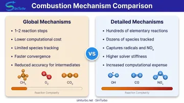
- Global mechanisms collapse chemistry into one or two steps (such as CH₄ + 2O₂ → CO₂ + 2H₂O). They cut cost but lose intermediate-species accuracy.
- Detailed mechanisms keep hundreds of elementary reactions and dozens of species. They can predict radicals, CO, and NOx, but add solver stiffness.
Arrhenius rate expressions set reaction speed: k = A exp(−Ea/RT), where Ea is activation energy, R is the gas constant, and T is temperature. Higher Ea makes the rate more temperature-sensitive, which creates stiffness and convergence trouble.
Stiff detailed mechanisms make chemistry integration expensive. In practice, engineers pick the simplest mechanism that still captures the outputs they need.
Types of Combustion Systems in CFD
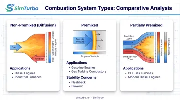
CFD combustion setups usually fall into three families: non-premixed, premixed, and partially premixed. The right family drives which scalars you solve and which closures you trust.
Non-Premixed (Diffusion) Combustion
Non-premixed flames form when fuel and oxidizer enter the reaction zone in separate streams and mix as they burn. The mixture fraction, a conserved scalar that tracks material from the fuel stream, is the main organizing variable.
Common applications include:
- Diesel-engine sprays, where liquid fuel vaporizes and mixes with air
- Industrial and utility furnaces firing natural gas or pulverized coal
- Liquid-spray and coal-particle cases in solvers such as ANSYS Fluent
Modern diesel engines often use partially premixed strategies, so calling every diesel case pure diffusion combustion oversimplifies real operation.
Premixed Combustion
Premixed flames form when fuel and air mix at the molecular level before ignition, then a flame front moves into the unburned mixture. Typical uses include port-fuel-injected gasoline engines and lean-premixed gas-turbine combustors.
Stability issues to watch in CFD and hardware alike:
- Flashback: flame travels upstream into the premixing zone
- Blowout: extinction under lean or high-velocity conditions
Homogeneous premixed flames are simpler to model than stratified systems. Real engines still show spatial gradients in equivalence ratio, so they often need richer closures than a single progress variable.
Partially Premixed Combustion
Hybrid systems blend premixed and non-premixed behavior to balance efficiency, emissions, and operability. Partially premixed models span the diffusion-to-fully-premixed range by carrying both mixture fraction and a reaction progress variable (as in ANSYS Fluent’s formulation).
GE’s LM6000 DLE (Dry Low Emissions) combustor work used a partially premixed laminar-flamelet approach on an ultra-low-emissions design. That matches how many modern gas turbines stage fuel injection and lean premixing to hold down NOx.
Major CFD Combustion Models Explained
Simple Chemical Reacting System (Finite Rate Chemistry)
This model solves transport equations for each species with Arrhenius kinetics, making it suitable for laminar or slow reactions. It is effectively exact for laminar flames, but inaccurate for turbulent flames if turbulence-chemistry fluctuations are ignored.
Computational expense rises steeply with mechanism size and stiffness. Finite-rate chemistry is appropriate when reaction timescales are comparable to or slower than turbulent mixing timescales, and when detailed intermediate species or ignition/extinction phenomena must be captured.
Eddy Dissipation Model (EDM) and Eddy Dissipation Concept (EDC)
EDM assumes fast chemistry with turbulent mixing as the rate-limiting step. Reaction rates are computed from the turbulent mixing time k/ε, making the model ideal for high-turbulence industrial flows where chemistry equilibrates faster than eddies mix. EDM is restricted to one- or two-step global reactions and cannot predict kinetically controlled radicals or minor species.
EDC extends EDM by assuming reactions occur in fine turbulent structures and integrating detailed Arrhenius chemistry in a reactor representation. That lets EDC use detailed mechanisms while staying mixing-controlled.
Stiff integration raises the cost, so EDC sits between EDM (cheap, limited chemistry) and full finite-rate methods (expensive, comprehensive chemistry).
Flamelet Models (Steady Laminar Flamelet and Flamelet Generated Manifolds)
Flamelet approaches represent turbulent combustion through laminar-flame solutions, commonly tabulated before or during CFD. NASA describes the table lookup as computationally inexpensive, and Siemens calls flamelet models quick and accurate within the flamelet regime.
Steady laminar flamelet pre-computes flame structure from one-dimensional laminar flame calculations at various strain rates. Those solutions map into the turbulent field through mixture fraction and scalar dissipation rate.
Flamelet Generated Manifolds (FGM) use multi-dimensional tables indexed by progress variable and mixture fraction. Chemistry collapses to a few lookup coordinates.
Limitations include departure from flamelet assumptions during extinction, reignition, or strong turbulence-chemistry interaction. Validation must confirm that the real flame behaves like an ensemble of laminar flamelets.
Probability Density Function (PDF) Models
PDF models close nonlinear turbulence-chemistry statistics by introducing a probability density function of mixture fraction, temperature, or composition. ANSYS Fluent uses an assumed-shape PDF (typically beta distribution) for its non-premixed combustion model, enabling statistical treatment of turbulent fluctuations without resolving them directly.
Cost and accuracy depend on whether the PDF shape is assumed or transported, and on how the chemistry table is built. In practice, PDF closures usually sit between eddy-dissipation simplicity and full finite-rate cost.
Conditional Moment Closure (CMC)
CMC solves species and enthalpy moments conditioned on mixture fraction or progress variable, giving higher fidelity than assumed PDF shapes. Cost stays moderate even with full mechanisms, though local extinction and reignition remain harder to validate.
CMC is most relevant to non-premixed flames where mixture-fraction conditioning organizes the flame structure, and where turbulent fluctuations significantly affect local reaction rates.
Model Comparison Summary
| Model | Computational Cost | Best Applications | Key Limitations |
|---|---|---|---|
| Finite Rate | High (scales with mechanism size) | Laminar flames, ignition, slow chemistry | Inaccurate for turbulent flames without closure |
| EDM | Low | Mixing-limited turbulent combustors | Restricted to global reactions, no intermediates |
| EDC | Moderate–High | Detailed chemistry in turbulent flows | Stiff integration costly |
| Flamelet | Low–Moderate | Flamelet-regime premixed/non-premixed | Breaks down under extinction, strong strain |
| Moderate | Non-premixed with turbulent fluctuations | Accuracy depends on assumed vs. transported PDF | |
| CMC | Moderate | Non-premixed with conditional structure | Limited extinction/reignition validation (historically) |
How to Choose the Right Combustion Model
Assess Your Combustion Type
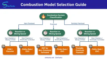
Start by classifying your system:
- Non-premixed: Use mixture-fraction-based models (flamelet, PDF, or non-premixed combustion)
- Premixed: Choose flamelet or EDM, depending on whether you need flame-front propagation detail
- Partially premixed: Use a model that retains both premixed and non-premixed limits, such as Fluent's partially premixed flamelet approach
Consider Reaction Speed vs. Mixing Speed
When reaction speed greatly exceeds mixing speed, chemistry equilibrates locally and combustion becomes mixing-limited. EDM or flamelet assumptions fit that regime well. When chemistry is slow or comparable to mixing, finite-rate or EDC models are needed to capture kinetic control, ignition delay, or local extinction.
Complex chemistry also matters when ignition delay and CO matter: matching mean temperature alone does not prove emissions accuracy.
Balance Accuracy and Computational Resources
Detailed chemistry (finite rate, EDC) delivers the best fidelity for intermediate species, ignition, and pollutants, but carries high computational cost. Simplified models (EDM, flamelet tables) run efficiently for engineering design when their assumptions match the physics.
Before committing to detailed kinetics, ask: Do I need radical concentrations, or is bulk heat release sufficient? Pick the cheapest model that still matches your regime and the outputs you must report. That choice yields the fastest design iterations.
Account for Emissions Prediction Needs
Predicting NOx, CO, and soot requires additional fidelity. CONVERGE documents dedicated thermal-NOx, PAH, and multiple soot treatments; ANSYS offers the Tesner soot model for radical nuclei and soot growth. Heat-release agreement does not guarantee accurate emissions, so species-specific validation is mandatory.
When emissions are design constraints, use finite-rate chemistry, EDC, or flamelet models with extended mechanisms, and check results against measured NOx, CO, and soot.
Practical Implementation Considerations
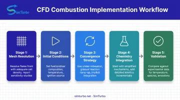
- Mesh resolution: Resolve the flame front with enough cell density. No universal combustion-cell size exists; an ASME engine study treats spray quantities that converge with refinement as the practical target. Report mesh and time-step sensitivity for flame location, pressure, temperature, and emissions, not residuals alone.
- Convergence: Use under-relaxation, gradual reaction-rate ramp-up, and implicit time integration for stiff chemistry. Converge simplified or reduced mechanisms first, then add detailed kinetics.
- Validation: In NASA's lean-direct-injection combustor case, near-injector errors traced mainly to spray injection and vaporization; downstream errors traced to subgrid mixing. Validate chemistry, turbulence, spray, and boundary conditions together, not the combustion model alone.
Real-World Applications of Combustion CFD Modeling
Aerospace Propulsion Systems
NASA modeled a lean-direct-injection combustor with approximately 862,000 cells and a five-species global mechanism. Temperature trends improved with a large-eddy-mixing treatment, though spray uncertainty limited accuracy.
GE Aviation evaluated CONVERGE for gas-turbine relight and combustor validation. Cases like these show how aerospace teams rely on combustion CFD for thrust optimization, fuel efficiency, and altitude performance.
NASA's 2008 high-fidelity injector work showed that CFD can improve injector design by evaluating performance sensitivity before hardware testing. The same approach extends to rockets: liquid-engine studies model fuel-oxidizer mixing, stability, and chamber pressure, while solid-motor simulations tackle time-accurate 3D flow and boundary-condition sensitivity for systems such as NASA's Space Launch System.
Once combustor CFD defines local flame and heat-release behavior, engineers still need full-engine cycle and control context. SimTurbo is a gas turbine system-simulation platform for that next step: architects can parameterize single-spool and dual-spool turbojets, afterburning cycles, and recuperated layouts, then run real-time performance and control studies on a standard PC.
Its J85-GE-21 validation matched NASA test data within ±2% for thrust, flow rate, temperature, and thrust-specific fuel consumption, which supports design trade studies and university research without treating the engine as a black box.
Automotive Internal Combustion Engines
Automotive CFD stacks chemistry, mesh adaptation, and emissions models before a single dyno pull. CONVERGE-type workflows commonly include:
- SAGE chemistry for gasoline, diesel, and alternative fuels
- Temperature-based adaptive mesh refinement for knock prediction
- Dedicated NOx and soot models
- Premixed models for port-fuel-injection gasoline engines
- Spray combustion models for direct-injection diesel systems
Engineers use these tools to tune piston-bowl geometry, injection timing, and air-swirl against emissions limits without giving up power or efficiency. Simulating in-cylinder combustion, heat transfer, and pollutant formation before dynamometer testing shortens development cycles.
Power Generation Gas Turbines
B&B-AGEMA used Siemens STAR-CCM+ reactive CFD and large-eddy simulation for a 100% hydrogen micromix combustor. Test-bench flames and NOx closely matched simulations, and the design target was below 35 ppm NOx at 50–100% load. Mitsubishi reports that high-precision combustion simulation supports its low-NOx natural-gas combustor design.
Flamelet and EDC models help utilities and OEMs design combustors that tolerate diverse fuels (natural gas, hydrogen blends, syngas) while meeting strict emissions limits. Teams also use combustion CFD to check:
- Flame stability across load points
- Pattern factor (exit temperature uniformity)
- Combustor liner heat load
Industrial Furnaces and Boilers
Riley Power used CFD on coal, oil/gas, and recovery-furnace systems and compared results with field performance. Babcock & Wilcox uses numerical modeling to assess air-jet penetration, mixing, char bed behavior, and combustion in kraft recovery boilers. The goal is higher efficiency and tighter pollutant control in process heating, waste incineration, and steam generation.
A 2022 peer-reviewed study developed a 2D CFD model for on-grate municipal-solid-waste incineration, representing the bed as porous media and coupling gas-phase combustion with solid-fuel conversion.
Advanced Concepts: Rotating Detonation and Scramjets
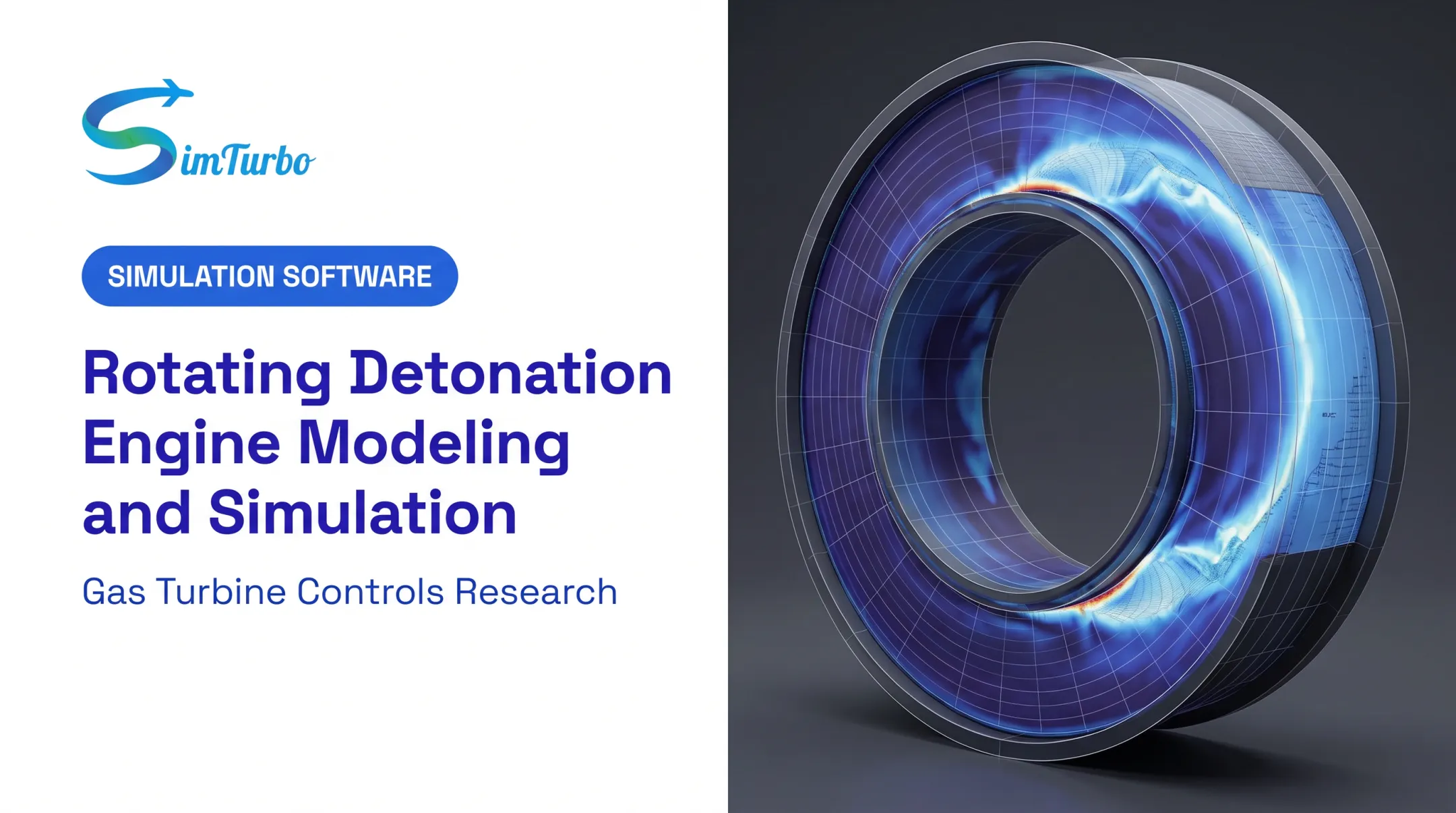
NASA's 2022 study ran 3D CFD parametric optimization on a laboratory rotating-detonation rocket-engine nozzle. That work is nozzle and flow-optimization evidence, not proof of a production engine. Rotating detonation combustors promise higher thermal efficiency through pressure-gain combustion, but they need transient CFD with detailed kinetics to capture detonation-wave propagation and coupling.
NASA's SCHOLAR scramjet validation case used 9 species and 18 reactions at a Mach 2 inlet. Computed and measured peak temperatures were about 2,030 K and 2,300 K, and CFD overpredicted primary-jet combustion. NASA and AFRL still flag a shortage of validation data for turbulent mixing and combustion closures at scramjet-relevant conditions, which is why experiment-linked validation remains essential at supersonic speeds.
Frequently Asked Questions
What is a combustion model?
A combustion model is a mathematical framework in CFD that represents chemical reactions, heat release, and species formation during fuel burning. It lets engineers predict flame behavior, temperature fields, and emissions without building physical prototypes.
What is CFD modeling used for?
CFD modeling simulates fluid flow, heat transfer, and chemical reactions in engineering systems. Combustion CFD predicts flame temperature, pollutants, fuel efficiency, and performance in jet engines, powertrains, boilers, and gas turbines.
How do I choose the right combustion model for my simulation?
Match the model to your regime (premixed, non-premixed, or partially premixed) and to whether mixing or chemistry limits the rate. Use EDM or flamelets for mixing-limited heat release; use finite-rate chemistry, EDC, or extended flamelets when ignition, extinction, or emissions matter.
What are common challenges in combustion CFD simulations?
Key challenges include achieving convergence with stiff chemical kinetics, resolving flame fronts with adequate mesh density, managing computational cost for detailed chemistry, and validating results against experimental data. Turbulence closure, spray vaporization, boundary conditions, and sparse validation data also limit accuracy.
How accurate are CFD combustion models?
Accuracy depends on model choice, mesh quality, chemistry fidelity, and validation. Well-validated flamelet or EDC setups can predict temperature and major species within about 5–10% when assumptions match the physics; minor species and emissions need detailed chemistry and measurement-based checks.
Which CFD software platforms support combustion modeling?
Major CFD platforms include ANSYS Fluent, Siemens STAR-CCM+, OpenFOAM, and CONVERGE (strong for internal-combustion engines). For gas-turbine system performance, transient operation, and control-law work alongside CFD, tools such as SimTurbo support component-based engine architecture and thermodynamic cycle analysis.
Next step: Pick the simplest combustion closure that matches your physics, validate early against data, and only add chemistry detail when temperature, species, or emissions targets require it.