Introduction
Internal Model Control (IMC) tuning is a model-based PID technique that uses a process model to calculate controller parameters for stable, robust control. Control engineers in aerospace, marine, and power systems often struggle with overshoot and instability when safety margins are tight.
IMC delivers predictable response without overshoot—critical for gas turbine engines, chemical reactors, and other high-value processes. Students gain a clear, systematic framework for controller design from the same approach.
This article covers IMC’s theoretical foundation, step-by-step tuning procedures, where it fits best, and when other methods make more sense.
Key Takeaways
- IMC tuning derives PID gains from a process model for stable control with minimal overshoot
- Needs process gain, time constant, and dead time from step testing, plus one closed-loop time constant
- Best for self-regulating processes (temperature, pressure, flow, speed) when stability beats speed
- One tuning parameter (closed-loop time constant) simplifies the speed-versus-stability trade-off
- May yield slow disturbance rejection on processes with very long time constants
What Is the IMC Tuning Method?
IMC tuning is a systematic way to calculate PID controller parameters from the internal model principle. That principle says effective control requires the controller to contain a representation of the process being controlled.
This model-based design produces controller settings with:
- Stable closed-loop response and minimal overshoot
- Predictable settling time
- Strong robustness to model uncertainty
Unlike trial-and-error tuning or aggressive methods like Ziegler-Nichols, IMC designs the controller from an explicit process model. Ziegler-Nichols targets quarter-amplitude damping—fast but oscillatory—while IMC prioritizes stability over speed.
The main advantage is one intuitive tuning parameter (the closed-loop time constant) instead of manually balancing multiple gains.
Why IMC Tuning Is Used in Process Control
IMC is adopted in industrial control applications because it provides stable control, eliminates overshoot that could damage equipment or trigger safety violations, and remains effective even when the process model is imperfect.
Process control applications demand:
- Predictable behavior during setpoint changes
- Consistent performance across varying operating conditions
- Robustness to disturbances
- Simplified tuning that shortens commissioning time
The cost of poor tuning: Per ISA guidance, weak closed-loop performance shows up in several ways:
- Deviation from setpoint
- Oscillation from incorrect tuning
- Instability when the loop is tuned for excessive speed
- Sluggish response, overshoot, or quality and equipment impact when loops are left poorly tuned
How IMC Addresses Model Uncertainty
IMC uses a conservative tuning approach based on the closed-loop time constant. Select a larger closed-loop time constant, and you build in robustness that holds stability even when the real process differs from the model.
That tradeoff favors reliable operation over aggressive speed. It is why IMC is valued in safety-critical work such as aerospace propulsion, pharmaceutical manufacturing, and energy generation, where overshoot or oscillation is unacceptable.
IMC is a strong fit when stability matters more than speed. Ziegler-Nichols typically yields a faster response with some overshoot; IMC aims for critically damped or overdamped behavior: slower, stable, and free of overshoot.
How the IMC Tuning Method Works
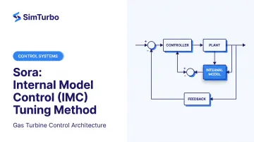
IMC assumes the controller holds an internal mathematical model of the process. It uses that model to predict future behavior and shapes the closed-loop response like a simple first-order filter with time constant τ_cl.
Key inputs to IMC tuning:
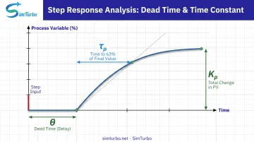
- Process gain (K_p): change in process variable per unit change in controller output
- Process time constant (τ_p): how quickly the process responds
- Process dead time (θ): delay before the process starts moving
- Closed-loop time constant (τ_cl): the user-selected knob that sets response speed
All of these parameters are obtained through step testing. The closed-loop time constant acts as the single tuning knob: larger values produce slower, more stable response; smaller values produce faster response but reduced robustness. A typical starting point is τ_cl = τ_p (matching the process time constant).
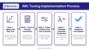
With those parameters in hand, the process model describes how controller output drives the process variable. IMC inverts that relationship to calculate the gains that deliver the closed-loop behavior you want. The steps below walk through the full procedure.
Step 1: Perform Open-Loop Step Test
Place the controller in manual mode and allow the process to settle at steady state. Make a 5-10% step change in controller output and record the process variable response over time until it settles at a new steady state. This test provides the raw data for extracting process parameters.
Step 2: Extract Process Parameters from Step Response
From the step response, extract:
- K_p: change in process variable (% of range) divided by change in controller output (%)
- θ: time from the step change to the first movement in the process variable
- τ_p: time for the process variable to reach 63% of its total change after dead time ends
If you prefer the graphical method, draw a tangent at the inflection point to read these values visually.
Step 3: Select Closed-Loop Time Constant
Choose τ_cl based on application requirements:
- Start with τ_cl = (1 to 3) × τ_p
- Use 2–3× τ_p when you want maximum stability and robustness
- Use 1–1.5× τ_p when you need faster response
- Keep τ_cl no smaller than dead time θ in most cases
Step 4: Calculate Controller Parameters Using IMC Equations
For a PI controller on a first-order-plus-dead-time (FOPDT) process, the IMC tuning formulas are:
K_c = τ_p / [K_p × (τ_cl + θ)]
T_i = τ_p
Use these with the non-interactive (parallel) PID algorithm. Setting integral time equal to the process time constant cancels process lag so the controller tracks setpoint changes smoothly.
Step 5: Implement and Validate Controller Settings
Enter the calculated values and confirm the controller is in non-interactive form. Then:
- Switch to automatic and apply a small setpoint change
- Check the response against your stability and speed targets
- Raise τ_cl for more stability, or lower it for faster response, if fine-tuning is needed
Where IMC Tuning Is Applied
IMC tuning is commonly used for:
- Temperature control – heat exchangers, reactors, ovens
- Pressure control – vessels, pipelines
- Flow control – feed streams, coolant loops
- Speed control – motors, turbines
- Composition control – chemical reactors, distillation columns
When IMC Tuning Occurs
IMC tuning typically occurs during:
- Initial commissioning of new control systems
- Re-tuning after process modifications or equipment changes
- Troubleshooting of unstable or poorly performing control loops
Engineers often choose IMC over other tuning methods when:
- Process safety requires no overshoot
- A process model is available or can be built from step tests
- Robustness to changing operating conditions matters
- Earlier aggressive tuning caused instability or heavy oscillation
IMC in Gas Turbine Engine Control Systems
On gas turbine engines, IMC-tuned PID loops are common for speed, temperature, and surge-margin control. Engineers can implement and validate those controllers in simulation before deployment in aerospace, marine, or power generation systems.
SimTurbo supports configurable PID controllers and real-time transient tests—startup, acceleration, and throttle changes—so tuning can be checked before it reaches the engine.
Key Factors That Affect IMC Tuning Performance
Three factors drive IMC tuning results in practice: model accuracy, operating-condition shifts, and your choice of closed-loop time constant.
Process Model Accuracy
IMC performance depends on how well the step test captures true process dynamics. Common sources of error include:
- Measuring dead time incorrectly on lag-dominant processes
- Performing step tests during periods of high disturbances
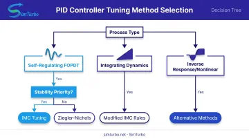
- Using a first-order-plus-dead-time model for processes with more complex dynamics (integrating, inverse response, higher-order)
Operating Condition Variability
Process gain, time constant, and dead time can change with flow rate, temperature, or pressure. IMC robustness helps maintain stability across moderate variability, but large changes may require gain scheduling or adaptive tuning.
Closed-Loop Time Constant Selection
τ_cl is the primary factor affecting control performance trade-offs:
- τ_cl = τ_p gives good balance for most applications
- τ_cl = 2-3 × τ_p maximizes robustness for uncertain or varying processes
- τ_cl < τ_p should only be used when faster response is essential and the process model is highly accurate

Common Issues and Misconceptions
A few recurring claims about IMC create confusion during controller design. Clearing them up helps you apply the method with the right expectations.
"IMC Always Produces Slower Control"
Reality: When τ_cl is set equal to τ_p, IMC often produces similar speed to properly tuned Ziegler-Nichols, but without overshoot. The perception of "slowness" comes from comparing IMC to aggressive Ziegler-Nichols tuning that sacrifices stability for speed.
"IMC Tuning Method" vs. "IMC Architecture"
Clarification: IMC tuning refers to the rules for calculating PID parameters. IMC architecture is a control structure with an explicit process model in the loop. You can apply the tuning rules to standard feedback controllers without implementing the full IMC architecture.
"IMC Requires a Perfect Process Model"
Reality: IMC is built to stay robust when the model is imperfect. Conservative τ_cl choices typically keep the loop stable despite model error. How much error you can tolerate depends on τ_cl relative to the process dynamics.
"IMC Integral Time Should Always Equal Process Time Constant"
Clarification: T_i = τ_p holds for first-order-plus-dead-time processes. Integrating processes and second-order systems often need modified IMC rules rather than that default equality.
When IMC Tuning May Not Be Appropriate
IMC suits many self-regulating loops, but some process types and control goals sit outside its strengths. Use a different method in the cases below.
Process Types Where Standard IMC Is a Poor Fit
- Integrating processes (such as liquid level control) that lack self-regulation
- Inverse-response processes with right-half-plane zeros
- Highly nonlinear processes where one linear model cannot cover the full operating range
Situations Where IMC Produces Slow Disturbance Rejection
Processes with very large time constant-to-dead-time ratios (τ_p >> θ) are a common weak spot. The constraint T_i = τ_p forces a long integral time, so disturbance-driven steady-state error clears slowly.
When Alternative Methods Are Better
Match the method to the objective:
- Fast setpoint tracking – use Ziegler-Nichols or lambda tuning with a very small λ
- Integrating dynamics – apply IMC-based rules built specifically for integrating systems
- Disturbance rejection over tracking – use a two-degree-of-freedom controller design
Conclusion
IMC tuning gives a model-based path to PID parameters that deliver stable, predictable control with minimal overshoot and solid robustness to process uncertainty.
The main lever is the closed-loop time constant. Tighten it for faster response; loosen it for more stability and robustness. That single choice is where most IMC tuning judgment sits.
IMC is not the best fit for every plant. Long time constants and integrating dynamics often call for another method. Match the tuning approach to the process, and control performance stays reliable.
Frequently Asked Questions
What is internal model control (IMC)?
IMC is a model-based control design philosophy where the controller explicitly contains a mathematical representation of the process. For PID tuning, it means equations that set controller gains from process gain, time constant, and dead time to get a stable, non-overshooting closed-loop response.
When should I use IMC tuning instead of Ziegler-Nichols?
Use IMC when stability and minimal overshoot are critical—such as safety-critical processes, expensive equipment, model uncertainty, or past instability from aggressive tuning. Use Ziegler-Nichols when fast response is the priority and some overshoot is acceptable.
What is a good closed-loop time constant to start with?
Start with τ_cl = τ_p (equal to process time constant) for a good balance between speed and stability. Increase to τ_cl = 2-3 × τ_p if the process model is uncertain or the process varies with operating conditions. Decrease cautiously toward τ_cl = θ only if faster response is essential and the model is accurate.
Does IMC tuning work for all types of processes?
Standard IMC tuning rules are designed for self-regulating (stable) processes with first-order-plus-dead-time dynamics, such as temperature, pressure, flow, and speed control. Integrating processes (like level control) and inverse-response processes require modified IMC tuning rules or alternative methods.
How accurate does my process model need to be for IMC tuning to work?
IMC tuning is deliberately robust to model errors and typically maintains stable control with reasonable model inaccuracies. Very small τ_cl values shrink that robustness margin, so larger model errors call for a more conservative closed-loop time constant.
Can I use IMC tuning with derivative action (full PID)?
IMC rules exist for full PID, but for first-order-plus-dead-time processes the gain over PI is usually small. Derivative action helps more on higher-order processes, at the cost of added complexity and noise sensitivity.