Thermodynamics of Turbines

Modern power generation, aerospace propulsion, and industrial systems all share one critical enabler: the gas or steam turbine. These machines extract mechanical work from high-temperature, high-pressure fluids with remarkable efficiency, but their performance is entirely governed by the fundamental principles of thermodynamics. Understanding how energy converts from pressure and temperature into shaft rotation—and why real turbines never reach theoretical perfection—requires a clear grasp of energy conservation, entropy generation, and the pressure-temperature relationships that define expansion through rotating machinery.

Whether you're analyzing a supercritical steam turbine in a baseload power plant or sizing a radial-inflow turbine for an aircraft APU, thermodynamics provides the essential framework. The First Law tells you how much work could come out; the Second Law explains why you won't capture it all. Isentropic expansion sets the benchmark, while pressure ratios, enthalpy drops, and velocity triangles translate those abstract properties into blade angles, stage counts, and thermal efficiencies. This article explores the thermodynamic principles that govern turbine operation, the cycles that frame their use, and the design decisions that balance ideal performance against real-world constraints.

---

Fundamental Thermodynamic Principles Governing Turbine Operation

First and Second Laws of Thermodynamics in Turbine Context

For a steady-flow, adiabatic turbine, the First Law of Thermodynamics reduces to a simple energy balance. Shaft work output per unit mass equals the drop in total (stagnation) enthalpy from inlet to exit:

w_s = h_t,in - h_t,out

Total enthalpy includes both the static thermodynamic state and the kinetic energy of the flow. Turbine work therefore comes from the fluid’s combined thermal and velocity energy. That is why calculations use total properties: bringing the flow isentropically to rest shows the full energy available for conversion.

The Second Law accounts for irreversibility. For an adiabatic turbine, entropy change equals internal entropy generation:

s_out - s_in ≥ 0

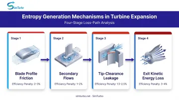
A reversible (isentropic) expansion would hold entropy constant. Real turbines always generate entropy through mechanisms such as:

• Blade profile friction and shock losses
• Secondary flows and endwall cross-flows
• Tip-clearance leakage
• Unrecovered exit kinetic energy

That entropy rise reduces available work. Energy that could have become shaft torque is lost to heat and mixing. The gap between ideal isentropic work and actual work is turbine efficiency, and it drives cycle performance, stage count, and cooling needs.

Isentropic Processes and Ideal Expansion

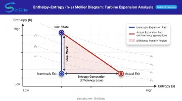
An isentropic expansion is the benchmark for turbine performance: a reversible, adiabatic process with constant entropy. On an enthalpy-entropy (h-s) diagram, it is a vertical line from the inlet state down to the exit pressure. The enthalpy drop on that path is the maximum work you can extract for a given pressure ratio.

Real machines do not reach that limit. Isentropic efficiency compares actual work to that ideal:

η_t = (h_in - h_out,actual) / (h_in - h_out,isentropic)

The numerator is the work you get; the denominator is the work a reversible expansion would deliver. Aircraft gas turbines and industrial steam turbines typically land near 90%, with validated ranges from 85% to 95% by machine class, size, and operating point. The shortfall traces to the same Second Law losses listed above.

Enthalpy-Entropy (h-s) Diagrams for Turbine Analysis

The Mollier diagram (h-s chart) makes those ideal-versus-actual paths visible. Vertical lines are constant-entropy processes; horizontal lines are constant-enthalpy mixing; pressure lines slope down and to the right. Plot an expansion from high to low pressure and the vertical drop is ideal work, while drift to the right (higher entropy) shows real losses.

How to read a turbine expansion on the chart:

• Inlet state: High pressure, high enthalpy
• Isentropic exit: Same entropy, lower pressure, lower enthalpy
• Actual exit: Higher entropy (further right), higher enthalpy than isentropic, so less work extracted

The horizontal gap between the two exit states is the efficiency penalty. For steam turbines in the two-phase region, quality lines also show moisture content (vapor versus liquid fraction), which matters for blade erosion and low-pressure stage efficiency.

Pressure and Temperature Relationships

For an ideal gas in isentropic expansion, pressure and temperature are tied through the specific heat ratio γ = c_p / c_v:

T_out / T_in = (p_out / p_in)^((γ-1)/γ)

That relation sets how much temperature drop, and therefore enthalpy drop, a given pressure ratio can deliver. Higher pressure ratios mean more work per stage, but they also need higher blade speeds or more stages to handle the velocity change.

Turbine pressure ratio (TPR) is inlet total pressure divided by exit total pressure. Typical stage capability looks like this:

• Single-stage axial turbine: about 2:1 to 3:1
• Radial-inflow turbine: 5:1 or more in one wheel (centrifugal work helps)
• Multi-stage machines: total ratio split across rows to limit loading and stay closer to reversible expansion

These ideal-gas relations assume constant specific heats. Gas turbines with inlet temperatures above about 1,500 K need variable c_p and γ or property tables. Steam turbines always need IAPWS steam tables, because water vapor is far from ideal near saturation.

Energy Balance and Work Extraction

The same steady-flow balance from the First Law still governs shaft work: total enthalpy drop from inlet to exit. In an axial turbine, that work comes from cutting the tangential component of absolute velocity as flow passes through the rotor. The Euler turbine equation states it directly:

w_shaft = U₁C_θ,in - U₂C_θ,out

Here U is blade speed and C_θ is the tangential (whirl) component of absolute velocity.

Stator nozzles accelerate the flow and aim it at the rotor. Rotor blades then turn and slow the whirl component, and that drop becomes shaft torque. Static temperature and pressure describe the local state only. Total properties add stream kinetic energy, so blade sizing and efficiency use total enthalpy and total pressure. Leave kinetic energy out and you understate available work and misread stage loading.

In practice, steady-state cycle models and stage-matching tools apply these balances row by row when you set pressure ratio, estimate isentropic efficiency, and check work split across the turbine.

Turbine Types and Their Thermodynamic Characteristics

Impulse Turbines: Nozzle-Driven Expansion

In an impulse turbine, all pressure drop occurs in stationary nozzles upstream of the rotor. The fluid exits the nozzles as a high-velocity jet at reduced pressure, then impacts the moving blades. Ideally, the rotor passages experience no further pressure drop: static pressure remains constant across the rotor row. This is called zero reaction (R = 0).

Confining expansion to the nozzles puts the rotor in a simpler flow field, with lower relative velocities and fewer aerodynamic losses from diffusion.

The tradeoff is exit kinetic energy. High absolute velocity into the rotor leaves substantial KE at the exit unless later stages or exhaust diffusers recover it—a major efficiency drain in single-stage impulse designs.

Velocity triangles for impulse stages are asymmetric: high absolute velocity in, lower absolute velocity out, with the rotor primarily redirecting the jet rather than expanding it.

Reaction Turbines: Continuous Expansion

A reaction turbine divides the pressure drop between stationary and rotating blade rows. The rotor passages themselves act as moving nozzles, accelerating the flow in the relative frame and dropping static pressure. 50% reaction is the most common design: half the stage's static enthalpy drop occurs in the stator, half in the rotor.

Continuous expansion allows more gradual velocity changes, which cuts profile losses from separation and shock. Aerodynamically active rotor passages can raise stage efficiency, and symmetric velocity triangles (equal inlet and exit angles) simplify repeated staging.

Because the rotor expands the flow, tip-clearance leakage and secondary flows matter more than in impulse stages. Tighter clearances and endwall contouring are critical to holding that efficiency.

Steam Turbines vs. Gas Turbines: Fluid Property Differences

Gas turbines typically operate with air or combustion products that behave approximately as ideal gases. Preliminary analysis uses constant γ ≈ 1.4 for air and γ ≈ 1.33 for hot combustion gases, with refinements for variable specific heats at high temperature. The working fluid remains single-phase throughout.

Steam turbines use water vapor, which shows strong real-gas behavior and often enters the two-phase region during expansion. Low-pressure stages may encounter moisture content (steam quality below 1.0), where liquid droplets form. This introduces several thermodynamic complications:

• Properties must come from IAPWS steam tables, not ideal-gas equations
• Wetness losses arise from droplet drag and blade erosion
• Enthalpy drop per stage is smaller in the two-phase region because latent heat buffers temperature change
• Reheat cycles limit exit moisture and improve efficiency

The same First and Second Law principles apply either way. Steam turbines need property lookups at every state point; gas turbines can often use closed-form isentropic relations with corrections.

Axial vs. Radial Flow Configurations

Axial turbines keep the flow path approximately parallel to the shaft. Blade speed U = ωr is nearly constant across the span, and each stage handles a modest pressure ratio (typically 1.5:1 to 3:1). Multi-stage axial machines are the norm for large power generation and aircraft engines because they scale efficiently to high mass flows.

Radial-inflow turbines turn the flow 90° inward, from a large-radius inlet to a smaller-radius exit. The Euler equation w = U₁C_θ,₁ - U₂C_θ,₂ shows that the large difference in blade speed (U₁ >> U₂) enables very high work per stage. One documented ASME case achieved a 5.7:1 pressure ratio and 87% total-to-static efficiency in a single wheel.

Choose the layout by duty:

• Radial: High pressure ratio, compact envelope, moderate mass flow (turbochargers, APUs, small gas turbines)
• Axial: Large mass flow, lower per-stage loading, multi-stage scalability (utility steam turbines, large jet engines)

Multi-Stage vs. Single-Stage Thermodynamic Considerations

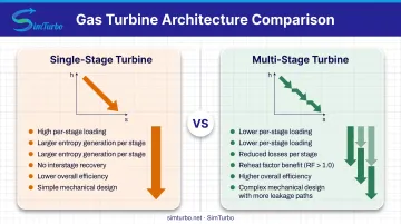
Dividing a large total pressure ratio into several smaller stages brings the expansion closer to reversible:

• Each stage operates at a lower loading, reducing losses from blade boundary layers and secondary flows
• Exit kinetic energy from one stage can partially recover as static pressure in the next stator
• Reheat factor (RF) captures diverging isobars on the h-s diagram: early-stage losses add enthalpy that later stages expand again, so RF = Σ(stage Δh_s) / (overall Δh_s) can exceed 1.0

More stages add weight, cost, and leakage paths. Power plants often run 20+ stages; aircraft engines keep stage count down to save weight.

Key Thermodynamic Cycles for Turbine Applications

The Rankine Cycle for Steam Turbines

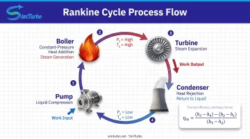
The Rankine cycle is the standard model for steam power plants:

1. Pump (1→2): Liquid water is compressed to boiler pressure (small work input)
2. Boiler (2→3): Constant-pressure heat addition vaporizes and superheats the steam
3. Turbine (3→4): Steam expands through the turbine, producing shaft work
4. Condenser (4→1): Exhaust steam condenses at low pressure, rejecting heat

Cycle efficiency:

η_th = (w_turbine - w_pump) / q_in = [(h₃ - h₄) - (h₂ - h₁)] / (h₃ - h₂)

A subcritical plant operating at 2,400 psig / 1,050°F / 1,050°F with single reheat achieves roughly 37–39% net efficiency (HHV basis).

A supercritical plant at 3,500 psig / 1,100°F / 1,100°F with reheat can reach 40–41% net efficiency, as documented in NETL reference case B12A.

Turbine's role: The turbine efficiency η_t directly sets the actual enthalpy drop h₄ = h₃ - η_t(h₃ - h₄s), which in turn determines cycle efficiency. Low turbine efficiency reduces net work and raises condenser heat rejection.

Brayton Cycle for Gas Turbines

The Brayton cycle governs gas turbines:

1. Compressor: Isentropic (ideal) or polytropic (real) compression raises air pressure and temperature
2. Combustor: Constant-pressure heat addition (fuel burn)
3. Turbine: Isentropic (ideal) or real expansion produces work
4. Exhaust: Heat rejection to atmosphere or to a nozzle (aircraft) or heat-recovery steam generator (combined cycle)

Ideal cycle efficiency (constant γ):

η_Brayton = 1 - (1 / r_p^((γ-1)/γ))

where r_p is the compressor pressure ratio. Higher pressure ratio raises ideal efficiency but also increases compressor work. The turbine must cover compressor work and still deliver net shaft output.

NASA matching equation:

• Compressor work: CW = c_p T_t2 (r_p^((γ-1)/γ) - 1) / η_c
• Turbine work: TW = η_t c_p T_t4 (1 - (1/r_p)^((γ-1)/γ))
• Shaft balance: TW = CW

Real-world consideration: Modern aircraft engines divert 20–30% of compressor flow to cool hot-section turbine blades. This cooling flow reduces the mass available for expansion and introduces mixing losses, so net efficiency is lower than the simple cycle formula suggests.

Ideal vs. Actual Cycle Performance

Ideal cycles assume:

• Isentropic compression and expansion
• No pressure losses in ducts or combustors
• Complete heat addition at constant pressure
• No mechanical or leakage losses

Real cycles include:

• Component efficiencies η_c and η_t (typically 85–95%)
• Combustor pressure loss (2–5% of inlet pressure)
• Mechanical losses (bearings, gearbox)
• Cooling and leakage flows

Example gap: An ideal Brayton cycle at pressure ratio 30 and peak temperature 1,600 K predicts about 55% thermal efficiency. A real engine with 90% component efficiencies, 3% combustor loss, and 25% cooling flow delivers closer to 40%.

Design work closes that gap through higher turbine inlet temperature, advanced coatings, and aerodynamic refinement.

Regenerative and Reheat Modifications

Regeneration (Rankine): Extract steam between turbine stages to preheat boiler feedwater. This reduces the fuel needed to reach the same final steam temperature, raising cycle efficiency by 3–5 percentage points. Each extraction point is called a feedwater heater.

Reheat (Rankine): After partial expansion, return steam to the boiler for additional heating, then expand again in a lower-pressure turbine. Reheat raises the average temperature of heat addition (improving efficiency) and prevents excessive moisture in the exhaust (protecting blades). Single reheat is standard; double reheat appears in the most advanced supercritical plants.

Recuperation (Brayton): Use hot turbine exhaust to preheat compressed air before the combustor. This reduces fuel consumption and can raise simple-cycle efficiency by 5–10 points, but adds weight and complexity, making it rare in aircraft and common in industrial microturbines.

Thermodynamic Optimization for Maximum Efficiency

Real turbine design balances competing objectives:

• Higher pressure ratio → higher ideal efficiency, but more compressor work, more stages, higher material stress
• Higher turbine inlet temperature → more available work, but greater cooling demand, advanced materials, coatings, and potential life reduction
• Extra stages cut per-stage loading and can lift efficiency, at the cost of weight, price, and more leakage paths

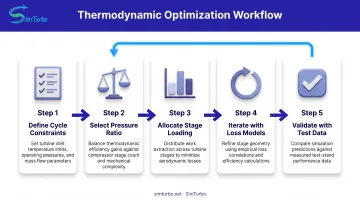
Optimization workflow:

1. Define cycle constraints: Inlet temperature limits (metallurgy), exhaust pressure (condenser vacuum or ambient), mass flow
2. Select pressure ratio: Trade ideal efficiency against compressor work and stage count
3. Allocate stage loading: Distribute total enthalpy drop to keep velocities reasonable and avoid separation
4. Iterate with loss models: Include profile, secondary, leakage, and exit kinetic losses; recalculate efficiencies and shaft power
5. Validate with test data: Benchmark predictions against rig tests or established engines

Engineers typically automate that loop in cycle-analysis software, sweeping design points until efficiency, matching, and durability constraints line up. Platforms such as SimTurbo support steady-state Brayton studies, compressor–turbine matching, and cycle options like recuperation so teams can test those trades before hardware.

Energy Conversion and Efficiency in Turbine Systems

Turbine Efficiency Definitions and Calculations

Isentropic efficiency remains the primary turbine performance metric:

η_t = (h_in - h_out,actual) / (h_in - h_out,isentropic)

Typical ranges:

• Industrial steam turbines: 88–92%
• Aircraft gas turbines: ~90% in advanced designs
• Small radial turbines: 85–87%

These values reflect the combined effect of all loss mechanisms (blade friction, shock, mixing, and leakage) under design operating conditions. Off-design operation (partial load, wrong speed) reduces efficiency further.

Polytropic efficiency measures efficiency over an infinitesimal pressure change, removing the influence of total pressure ratio:

T_out / T_in = (p_out / p_in)^(η_poly (γ-1)/γ)

Polytropic efficiency is more consistent across machines with different pressure ratios, making it useful for comparing turbine families. However, it requires iterative calculation and is less intuitive than isentropic efficiency.

Losses and Irreversibilities in Turbine Expansion

Every deviation from isentropic expansion generates entropy and reduces work:

• Profile losses: Boundary layers, wakes, and shock waves (transonic stages) consume energy; thinner layers and well-shaped airfoils cut these losses
• Secondary-flow losses: Endwall vortices form where blade pressure gradients meet the hub or casing; cross-passage mixing raises entropy downstream
• Tip-leakage losses: Clearance flow bypasses the blade row and mixes with the main stream; tight clearances and shrouds (where practical) limit leakage
• Trailing-edge and cooling losses: Thick edges and ejected cooling air create wakes and temperature/velocity mismatches that mix out as entropy
• Exit kinetic energy: High exhaust velocity leaves unused kinetic energy; diffusers recover some static pressure, but full recovery is impossible

In well-designed turbines, profile and secondary losses dominate at design point. Tip leakage becomes critical in small machines (large clearance-to-span ratio) and at high Mach numbers, where the leakage jet can choke.

Euler Turbine Equation and Work Output

The Euler turbine equation connects fluid mechanics to thermodynamics:

w_shaft = U₁C_θ,in - U₂C_θ,out

• U = blade speed (ωr)
• C_θ = tangential component of absolute velocity

Physical meaning: Work extraction equals the change in angular momentum per unit mass. Stator nozzles impart swirl (C_θ,in); the rotor removes it (C_θ,out drops). The product of this swirl change and blade speed is the work done on the shaft.

Design implication: To maximize work, designers raise blade speed (higher rpm or larger radius) and set flow angles to maximize ΔC_θ. Higher velocities also raise Mach numbers, shock losses, and stress, so a practical ceiling applies.

That is why high-work stages use large-diameter rotors or radial inflow (large U difference), while moderate-work stages stack multiple axial rows.

Practical Applications and Design Considerations

Software Tools for Thermodynamic Analysis

Modern turbine engineers rely on simulation software to model complex expansion processes, predict performance across operating ranges, and optimize designs before physical prototyping. These tools solve the coupled thermodynamic, fluid-dynamic, and mechanical equations that define turbine behavior, often using component maps, real-gas properties, and loss correlations validated against test data.

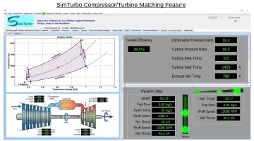
SimTurbo is a gas turbine simulation platform for real-time thermodynamic analysis of turbojet, turbofan, and related configurations. Its component-based architecture lets engineers assemble and re-parameterize engines by dragging and dropping inlets, compressors, combustors, turbines, nozzles, shafts, recuperators, and afterburners.

The software solves steady-state and transient Brayton-cycle equations with standard thermodynamic relations, gas-property tables, real-gas effects, and pressure-loss modeling.

Key capabilities for turbine thermodynamics:

• Interactive T–S and P–V diagrams that update live as compression, heat addition, and expansion paths change
• Turbine and compressor maps showing corrected mass flow, pressure ratio, and efficiency for shaft-work matching
• Steady-state curves for thermal efficiency and TSFC (e.g., efficiency from 0.1 to 0.5 across 4,000–20,000 RPM)
• Transient runs for startup, throttle bursts, afterburner ignition, and FADEC response, including TIT, surge margin, and entropy generation
• Time-series export (RPM, EGT, thrust, SFC) to CSV or Excel for MATLAB, Simulink, or Python

SimTurbo also supports advanced configurations such as recuperated cycles, reheat, and afterburners, allowing engineers to assess cycle efficiency improvements thermodynamically. Its physics-informed neural network control logic helps hold turbine inlet temperature limits while preserving compressor surge margin during safe, efficient operation.

In the classroom, the same models help students trace Brayton-cycle paths, see where entropy is generated, and link textbook relations to engine behavior in propulsion courses, labs, and capstone projects.

Real-World Performance Examples and Validation

Benchmark studies compare simulation results against measured performance from test stands or operational engines. That comparison quantifies prediction accuracy and refines loss models.

NASA J85-GE-21 validation: SimTurbo's single-spool turbojet model was checked against NASA Lewis Research Center test data for the J85-GE-21 and matched thrust, flow rate, temperature, and TSFC within ±2%. Component-based modeling paired with validated turbine and compressor maps produced that agreement across the operating envelope.

Typical operating parameters:

• Industrial steam (utility): inlet 3,500 psig / 1,100°F, reheat to 1,100°F, exhaust ~1 psia, multi-stage LP with moisture under 10%
• High-bypass turbofan: compressor PR 40–50:1, TIT 1,600–1,700 K, core turbine efficiency ~90%, 20–30% of core flow used for cooling
• Small radial turbines (APU, turbocharger): PR 3:1 to 6:1, single stage, efficiency 82–87%, compact envelope

These examples show the wide range of thermodynamic conditions turbines must handle—from saturated steam at near-vacuum to 1,700 K combustion products at 50 bar. Each case needs the right property model: steam tables, ideal gas, or real gas.

Design Trade-offs and Engineering Decisions

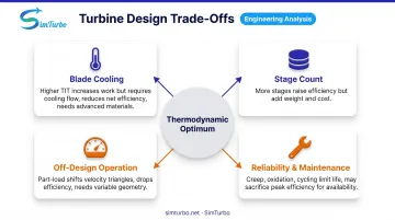
Thermodynamic analysis informs—but does not alone dictate—design. Engineers must balance efficiency goals with practical constraints:

• Blade cooling: Higher TIT raises available work but needs film cooling, internal convection, or TBCs; cooling flow cuts net efficiency, and materials (nickel superalloys, single-crystal castings, ceramics) set temperature limits and cost
• Stage count: More stages lower loading and raise efficiency, yet add weight, length, and parts—aircraft engines cut stages for weight; power plants accept 20+ stages for peak efficiency
• Off-design operation: Part load shifts velocity triangles, raises losses, and drops efficiency; variable geometry and fuel scheduling help, but thermodynamic limits remain
• Reliability and maintenance: Creep, oxidation, thermal cycling, and moisture erosion cap life; base-load plants often trade peak efficiency for longer overhaul intervals and higher availability

Thermodynamic optimization points to the theoretical best layout. Engineering judgment then picks the configuration that meets cost, weight, safety, and life-cycle targets for the actual mission.

Frequently Asked Questions

What are the four main types of turbines?

The four primary types are steam, gas, hydraulic, and wind turbines. Steam and gas turbines use thermodynamics to turn high-temperature, high-pressure fluid expansion into shaft work (Rankine and Brayton cycles, respectively).

What is the Euler turbine equation?

The Euler turbine equation states that work per unit mass equals the change in tangential velocity component times blade speed: w = U₁C_θ,₁ - U₂C_θ,₂. It describes how angular momentum transfer in turbomachinery translates thermodynamic enthalpy drop into shaft torque, guiding blade angle and velocity triangle design.

What is the difference between impulse and reaction turbines?

Impulse turbines convert all pressure energy to kinetic energy in stationary nozzles before the rotor, resulting in zero reaction (no rotor pressure drop). Reaction turbines feature continuous pressure drop across both stationary and rotating blade rows, typically with 50% reaction assigning half the stage enthalpy drop to the rotor.

How does the Rankine cycle relate to turbine efficiency?

The Rankine cycle is the thermodynamic framework for steam turbine power plants. Turbine isentropic efficiency η_t sets the actual enthalpy drop (h₃ - h₄), so higher η_t raises net cycle work and cuts fuel use per kWh.

What is isentropic efficiency in turbines?

Isentropic efficiency is the ratio of actual turbine work to ideal work from reversible adiabatic expansion at the same exit pressure: η_t = (h_in - h_out,actual) / (h_in - h_out,isentropic). It typically ranges from 85–95% depending on turbine type, size, and operating conditions, with modern aircraft turbines achieving approximately 90%.

How do pressure and temperature ratios affect turbine performance?

Higher pressure ratios raise work potential per stage but need more stages or higher tip speeds to handle the velocity change. Inlet temperature sets how much work you can extract; material limits (creep, oxidation) cap peak conditions and often force cooling and coatings.