Get it wrong on an industrial oven and you waste energy. Get it wrong on a gas turbine engine control and you risk compressor surge or a failed test run. This guide walks through what each PID term does, a manual tuning sequence engineers actually use, the Ziegler-Nichols method and its limits, common mistakes, and how simulation tools help you validate tuning before it ever touches hardware.
Key Takeaways
- Three PID terms each correct a different error component: present (P), accumulated (I), and rate of change (D)
- Manual tuning works best in sequence — proportional first, then integral, then derivative
- Ziegler-Nichols gives a fast starting point but typically produces aggressive, oscillatory results
- Simulate the loop before hardware testing to catch issues early and shorten validation
What Does PID Stand For and What Is It Used For?
PID stands for proportional-integral-derivative: a feedback control method that continuously compares a setpoint against the measured process variable and adjusts an output to close the gap. The International Society of Automation calls PID the most common industrial control technology in use today.
PID loops show up almost everywhere a process needs to hold steady:
- Temperature control in furnaces, ovens, and reactors
- Pressure and flow regulation in pipelines
- Motor speed and position control
- Gas turbine engine parameters like RPM, exhaust temperature, and surge margin
Not every application needs all three terms. Engineers regularly run P-only or PI control when derivative action would amplify noise more than it helps. A well-tuned PI loop handles many real-world processes without D at all.
Understanding PID Parameters: What Do Kp, Ki, and Kd Do?
Each gain term shapes the response differently, and knowing which knob does what is the foundation of tuning.
Kp (proportional gain) produces correction proportional to the current error. Push it higher and rise time drops, but you introduce more overshoot. According to University of Michigan's Control Tutorials for MATLAB and Simulink, increasing Kp decreases steady-state error too, but rarely eliminates it entirely.
Ki (integral gain) accumulates error over time to wipe out that remaining steady-state offset. The tradeoff: too much Ki causes overshoot and settling delays. If the actuator saturates, the integrator keeps accumulating error it cannot act on. That condition, integral windup, can drive a large overshoot once the loop finally recovers.
Kd (derivative gain) reacts to how fast the error is changing, damping oscillations and improving stability. The catch is that derivative action amplifies noise, so NI's PID theory guide recommends using it cautiously on noisy measurements.
| Gain | Rise Time | Overshoot | Settling Time | Steady-State Error |
|---|---|---|---|---|
| Kp ↑ | Decreases | Increases | Small change | Decreases |
| Ki ↑ | Decreases | Increases | Increases | Eliminated |
| Kd ↑ | Minor change | Decreases | Decreases | No effect |

These are general tendencies, not guarantees. CTMS notes they do not hold for every system, so verify with your own step tests.
One rule you can't skip: polarity. The process gain and controller gain must have opposite signs so the loop produces negative feedback. If a fuel valve opening increases speed, the controller must reduce output as speed rises above setpoint. Otherwise the loop drives itself further from target instead of correcting. Confirm this experimentally before you tune anything else.
Step-by-Step Manual PID Tuning Method
Manual tuning is slower than a formula, but it gives you a controller that actually behaves the way your process needs.
Step 1: Verify the sign of process gain. Bump the manipulated variable and confirm the process moves in the expected direction. If it moves opposite, reverse the controller action before touching any gains.
Setting the Proportional Term
Start with a low Kp and run setpoint step tests. Gradually increase the gain while watching the response.
- Increase Kp incrementally, testing after each change
- Watch for a slight overshoot that settles quickly: that's your target
- Stop before the response oscillates persistently
Adding the Integral Term
Introduce integral action starting with a large integration time, meaning sluggish I-action.
- Begin with a slow (large) integral time constant
- Decrease it gradually, running a step test after each adjustment
- Watch for oscillation starting to creep in
- Back off once you see the first sign of instability
Adding the Derivative Term (If Needed)
A well-tuned PI loop is often good enough. Many industrial processes never need D at all.
If you do add derivative action:
- Start with a small derivative time, roughly one-tenth the integral time
- Increase it cautiously, watching for noise amplification
- Stop as soon as the response gets jittery instead of smoother
Robustness tradeoff: Aggressive tuning gets a faster response, but it is often less robust when conditions change. A loop tuned tight at partial load may misbehave at full load, a pattern turbine and aerospace engineers see constantly.

Ziegler-Nichols Method: How It Works and Its Limitations
Ziegler-Nichols is the classic shortcut for getting a rough starting point fast.
The process:
- Disable integral and derivative action
- Increase Kp until the loop oscillates with constant amplitude
- Record the ultimate gain (Ku): the proportional gain at that oscillation point
- Record the ultimate period (Tu): the time for one full oscillation cycle
- Plug Ku and Tu into the standard Ziegler-Nichols formulas to get starting P, I, and D values
| Controller | Kp | Ti | Td |
|---|---|---|---|
| P | 0.5 Ku | — | — |
| PI | 0.45 Ku | Tu / 1.2 | — |
| PID | 0.6 Ku | Tu / 2 | Tu / 8 |
The catch: this method often produces loops that are too aggressive for real-world use. A peer-reviewed reassessment published in the Journal of Process Control found that the classic rules were correlated against simple step-response features and often lead to poor robustness. The resulting loop oscillates more than most processes can tolerate.
Treat Ziegler-Nichols as a rough starting point, not a finished answer. Run the numbers, then refine manually or validate in simulation before committing to hardware.

Common PID Tuning Mistakes
Even experienced engineers fall into these traps:
- Tuning all three terms at once. This makes it nearly impossible to isolate which gain caused an unstable or oscillatory response. Tune sequentially instead.
- Ignoring integral windup. When the actuator saturates, an unchecked integrator keeps accumulating error and drives large overshoot on recovery. Use anti-windup (back-calculation or conditional clamping); MathWorks covers both in its anti-windup control guide.
- Tuning at one operating point only. A loop tuned at 50% load may behave differently near full throttle. Nonlinear systems like gas turbines shift fuel-feed dynamics across the operating envelope, a familiar challenge in aircraft engine control.
Validating PID Tuning Through Simulation Before Deployment
Testing tuning changes directly on running hardware is expensive and risky, particularly on a turbine engine where a bad gain can mean surge or overtemp. Simulation lets you screen for these problems first.
SimTurbo is a gas turbine engine simulation platform built for this kind of virtual validation. Its component-based interface includes built-in PID blocks (Speed PID, Temperature PID, and Surge Margin PID), plus limiter logic and FADEC controls, all running in real time on a standard PC.
You can stress-test tuning across conditions like:
- Startup and shutdown sequences, slam-acceleration, and throttle transients
- Load changes, actuator response, and sensor-failure scenarios
- Compressor stall or surge events, including surge-margin drops from a normal 20–25% range down below 5%
- Steady-state design-point and off-design performance across altitude and ambient conditions
SimTurbo's steady-state outputs are benchmarked against NASA Lewis Research Center test data for the J85-GE-21 turbojet, reporting agreement within ±2% for thrust, flow rate, temperature, and fuel consumption. That gives engineers a credible reference point when judging whether their simulated tuning behavior is realistic.

Once a control law looks solid in simulation, export transient data (RPM, EGT, thrust, and SFC) to CSV or Excel for further analysis. PID or FADEC responses can also ship out as plant models for control laws built in MATLAB/Simulink or Python, then move toward test-cell hardware.
The same workflow helps university capstone teams learning control tuning for the first time. Discounted student licensing and classroom/lab programs let students tune, break, and re-tune a virtual PID loop without risking real equipment.
For a class project or research build, start with the 30-day free trial and run the workflow yourself.
Frequently Asked Questions
What does PID stand for and what is a PID controller used for?
PID stands for proportional-integral-derivative, a feedback control method that continuously calculates the error between a setpoint and a measured process variable. It's used across industrial and aerospace applications, including temperature, pressure, flow, motor control, and turbine engine management.
What do Kp, Ki, and Kd do in a PID controller?
- Kp: Reacts to current error and speeds up response, but adds overshoot
- Ki: Eliminates steady-state error by accumulating past error; too much causes overshoot and windup
- Kd: Dampens oscillation by reacting to the error's rate of change, but can amplify sensor noise
What is the Ziegler-Nichols method for tuning PID controllers?
It's a heuristic method: raise proportional gain until the loop oscillates at constant amplitude. Use that ultimate gain and period to calculate starting P, I, and D values. It's fast but often produces aggressive, oscillatory tuning that needs refinement.
What are common PID tuning mistakes?
The most common mistakes are:
- Tuning all three gains at once instead of sequentially
- Ignoring integral windup after actuator saturation
- Tuning at one operating point and assuming it holds across the full range
Is PID control still used?
Yes. PID remains the dominant control method in industry because of its simplicity, reliability, and effectiveness, even as more advanced control strategies like model-predictive control gain traction in complex systems.