Introduction
Gas turbine engineers have to choose what a simulation is for: the equilibrium state, or the dynamics that get you there. That choice drives run time, compute cost, result accuracy, and which insights you can trust.
Transient and steady-state analysis answer different questions. Steady-state tells you "how much" at equilibrium. Transient tells you "how fast" during startup, a throttle change, or a load shed. Pick the method that matches the objective: mapping an operating envelope, or validating control response under rapid change.
This guide compares both approaches, lays out practical selection criteria, and gives a simple decision framework for gas turbine performance analysis.
Key Takeaways
- Steady-state sets time derivatives to zero so differential equations become algebraic equilibrium solves
- Pressures, temperatures, shaft speeds, and flows evolve over time only in transient analysis
- Fewer properties and faster convergence make steady-state ideal for design optimization and performance maps
- Thermal mass, inertia, and time-step data are required to expose dynamic engine behavior
- Use steady-state for operating points and design exploration; use transient for startups, control validation, and time-critical events
Steady State vs Transient: Quick Comparison
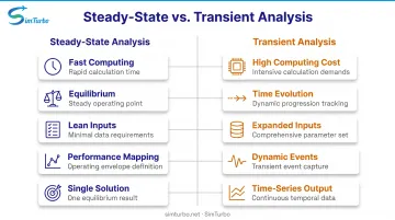
Use this side-by-side view to match analysis type to your design question—equilibrium performance versus time-dependent behavior.
| Attribute | Steady State | Transient |
|---|---|---|
| Computational Cost | Lower demand, faster solves; fits iterative design loops | Higher cost, longer runs; needs time-stepping and per-step convergence |
| Time Information | No real-time link; results show equilibrium only | Needs real-time specs; tracks system evolution over time |
| Model Inputs | Lean set: conductivity, flow data, component maps | Expanded set: specific heat, thermal mass, inertia, rotor moments, inter-component volumes |
| Typical Applications | Performance maps, design points, efficiency, sizing, parametric sweeps | Startup/shutdown, control validation, thermal cycling, emergencies, throttle transients |
| Results Output | One equilibrium solution for final operating conditions | Time-series from initial conditions to final state |
What is Steady-State Analysis?
Steady-state analysis is a modeling approach where all system variables—pressures, temperatures, flow rates, shaft speeds—have reached equilibrium and no longer change with time. Mathematically, all time derivatives (d/dt) equal zero, so differential equations simplify to algebraic equations that solve faster.
Most gas turbine performance work focuses on relatively constant operating points such as cruise power, idle, or base load. Steady-state analysis answers questions about thrust, efficiency, fuel consumption, and component matching at those equilibrium conditions.
"Steady state" does not mean the system is static. Turbines still spin, fuel flows, and gases move through the engine; those quantities simply hold constant average values over time. It also does not mean the engine started that way. Steady state is the long-term equilibrium after initial transients have died out.
Key Benefits of Steady-State Analysis
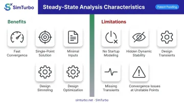
When the operating point is stable, steady-state models deliver equilibrium performance with far less computational overhead.
- One converged nonlinear matching solution per operating point
- Boundary conditions only (ambient pressure, temperature, flight Mach number)—no initial conditions, time steps, or time-integration logic
- Component maps supply off-design flow, pressure ratio, speed, and efficiency
- Convergence criteria apply to a single point, not a time history
That speed makes steady-state a workhorse in early design. You can sweep hundreds of configurations, build performance maps across altitude, Mach number, and power setting, and run geometry or materials trades before investing in detailed transient work.
Limitations of Steady-State Analysis
Equilibrium assumptions break down whenever time derivatives matter.
Startup and shutdown sit outside the model:
- Cold-start thermal stresses stay invisible
- Emergency-shutdown pressure transients are not modeled
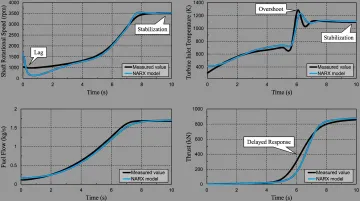
- Shaft acceleration, fuel-flow ramp-up, and temperature overshoot or lag do not appear
Dynamic stability problems stay hidden as well. You get surge margin at equilibrium, not surge cycles; combustion instabilities and control oscillations or governor hunting will not show up; rotating stall needs time-resolved modeling.
Some systems never truly settle. Certain combustion processes, persistently unsteady separation, and low-power or windmilling regimes may lack a stable equilibrium. Non-convergence or oscillating residuals are often the cue to switch to transient analysis.
What is Transient Analysis?
Transient analysis is time-dependent modeling that shows how system variables move from one state to another over real elapsed time. It keeps the full differential equations—and their time derivatives—and advances the solution with numerical integration at discrete time steps.
That matters for gas turbines because engines spend a lot of operating time accelerating, decelerating, and reacting to disturbances. You need transient simulation to see how fast the engine reaches a new point, whether limits are crossed on the way, and how the control system responds.
Unlike steady-state analysis, which solves straight for equilibrium, a transient run needs a defined starting point. That might be a cold engine at ambient, a hot engine at idle, or any state in between—without it, the path forward is undefined.
Time-step choice sets the tradeoff between fidelity and cost. NASA’s 1974 DYNGEN guidance suggested a step about one-tenth of the smallest time constant of interest—so a rotor with a 1.0 s time constant points to steps no larger than 0.10 s. Smaller steps raise accuracy and cost; larger steps can skip real dynamics or go numerically unstable.
Key Benefits of Transient Analysis
Transient runs expose dynamics you cannot see at equilibrium:
- Time scales of competing physical processes, including thermal lag behind shaft acceleration
- Throttle, governor, and safety-system timing under realistic load changes
- Fuel scheduling against speed and temperature limiters during fast transients
- Temperature overshoot, startup pressure oscillations, and thermal cycling fatigue
- Surge-margin excursions on afterburner engagement (documented drops from 20–25% to below 5%)
- Fuel-system delays that lag engine response by 0.5 s or more
Control design depends on this view. It is also a certification issue: FAA 14 CFR 33.73 requires engines to reach 95% rated takeoff power within 5 seconds from flight idle.
Limitations of Transient Analysis
Those gains come with real cost. Each step must converge the nonlinear component equations before time can advance, so runtime scales with duration, tighter steps, and model detail. In one 1974 NASA case, a 3-second transient took 1.4 minutes at 0.10 s steps and 12.3 minutes at 0.01 s steps. High-fidelity models today can still run for hours or days.
Setup is heavier than steady-state work:
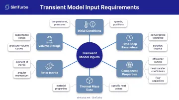
- Initial conditions for every state variable
- Time-step size and convergence tolerance matched to the dynamics
- Duration long enough to capture the event of interest
- Extra inputs such as rotor inertia, inter-component volumes, and design speeds
You also need more property data—thermal mass and specific heat for thermal transients, rotating inertia for shaft dynamics, plus bulk modulus, density, and storage volumes for fuel and inter-component flow.
Steady State vs Transient: Which Should You Use?
Match the method to the question you need answered. Use steady-state for "how much" or "what value at equilibrium." Use transient for "how fast" or "when does it reach" a target condition.
Those criteria map directly to common engineering objectives:
| Engineering Objective | Recommended Method |
|---|---|
| Design point performance | Steady-state |
| Operability limits and surge margin | Steady-state |
| Component sizing and matching | Steady-state |
| Startup time and sequence | Transient |
| Control response and stability | Transient |
| Thermal cycling and fatigue | Transient |
| Acceleration/deceleration schedules | Transient |
Situational Recommendations for Gas Turbine Engineers
Choose steady-state when you need to:
- Map performance across the operating envelope (altitude, Mach number, power setting)
- Size components for target efficiency or thrust
- Optimize geometry for maximum performance or minimum fuel consumption
- Generate compressor or turbine performance maps
- Conduct parametric studies with dozens or hundreds of design variations
When timing, dynamics, or control response drive the decision, switch to transient analysis.
Choose transient when you need to:
- Validate startup sequences and windmilling-to-idle transitions
- Design acceleration and deceleration schedules
- Evaluate control system stability and response time
- Assess thermal stress during mission profiles
- Predict time to reach operating temperature
- Verify compliance with FAA response requirements (5 seconds to 95% rated takeoff power)
Consider a hybrid approach:
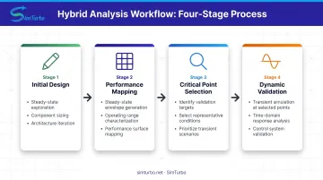
Most programs get better results by sequencing both methods:
- Use steady-state for initial design and rapid exploration of the design space
- Run transient simulations for final validation at critical operating conditions
- Initialize transient runs from converged steady-state solutions to reduce setup complexity
- Generate steady-state performance decks, then validate selected points with transient analysis
Common Pitfalls to Avoid
Attempting steady-state on inherently unsteady problems:
- Warning signs include residuals that oscillate rather than converge
- Solution variables that drift or cycle rather than settling
- Operating points outside the coverage region of component maps
- Sub-idle conditions where nonlinear models can become unstable
Under-resolving transient simulations:
- Time steps that are too large miss important dynamics
- Insufficient resolution can introduce numerical instability
- Symptoms include non-physical oscillations, sudden jumps in variables, or divergence
- NASA DYNGEN saw nearly identical results at 0.10 s and 0.01 s in one case; size steps to the fastest dynamics you retain
Ignoring computational budget:
- Estimate simulation costs before committing to transient analysis of large systems
- Balance fidelity with available time and computing resources
- Consider whether the engineering decision justifies the added cost
- Remember that transient cost grows with duration, step count, and model complexity
Real-World Applications in Gas Turbine Simulation
Gas Turbine Startup: Transient Analysis Essential
Startup work is a classic transient problem:
- Engine acceleration from windmilling to idle captures shaft speed ramp-up
- Fuel flow scheduling must be validated to avoid overtemperature or flameout
- Temperature rise through combustor and turbine lags mechanical acceleration
- Time to reach a stable operating point drives mission readiness
- Controls must manage fuel flow, variable vanes, and bleed valves dynamically
Startup simulations need compressor and turbine maps extended to 5–10% corrected design speed—well below normal idle-to-full-power coverage. Rotor inertia and inter-component volumes become critical inputs.
A restart model for a 40,000 lbf-class turbofan tracked an 80-second purge and acceleration-to-idle sequence. It captured high-pressure-shaft relight thresholds and windmilling dynamics.
Performance Mapping: Steady-State Excels
Performance decks across flight conditions favor steady-state methods:
- Altitude, Mach, and power-setting combinations can number in the hundreds or thousands
- Each point needs converged thrust, fuel flow, temperatures, and component operating lines
- Steady-state analysis delivers those results without time-stepping
- Decks support mission analysis, range calculations, and propulsion integration
An F100 flight-thrust deck study measured 20 aircraft and 18 engine parameters across light, medium, and heavy configurations in both dry and afterburning regimes. Running transient simulation at every point would be impractical.
Control System Validation: Transient Analysis Required
Throttle response and limit protection are transient problems:
- FAA 14 CFR 33.73 requires engines to reach 95% rated takeoff power within 5 seconds from flight idle
- A power-lever slam from minimum to maximum in 1 second or less must not cause overtemperature, surge, stall, or other damage
- Controls must enforce shaft-speed limits, turbine-inlet-temperature limits, and surge-margin protection
- Fuel scheduling, variable geometry, and bleed control must stay coordinated in real time
Transient simulation exercises acceleration schedules, limit logic, actuator dynamics, and sensor response. A Cranfield fuel-system integration study found fuel-system delays lagged engine response by about 0.5 seconds—enough to require modeling the full control loop.
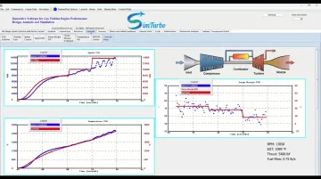
SimTurbo: Integrated Steady-State and Transient Simulation
SimTurbo supports transient and steady-state gas turbine analysis in one environment, so the same model can move from performance mapping to dynamic validation.
Real-time transient simulation on standard PCs:
- Interactive views of throttle effects, temperature evolution, and shaft dynamics as they happen
- Time-history graphs, component maps, and cycle diagrams that update in real time
- Live RPM, EGT, thrust, and surge-margin trends during startup, acceleration, and load changes
Component-based architecture:
- One model for steady-state performance mapping and transient control validation
- Inlets, compressors, combustors, turbines, nozzles, shafts, sensors, actuators, PID controllers, and FADEC logic on a design palette
- Steady-state points across the flight envelope, then transient runs to check control response—without rebuilding the model
Practical workflow: A university capstone team or aerospace engineer can map steady-state performance across altitude and Mach, size components for target thrust and efficiency, then validate startup and throttle response with transient runs started from those solutions.
Transient data (RPM, EGT, thrust, SFC) exports to CSV or Excel for post-processing. Built-in PID and FADEC logic can also export for external control-law checks.
SimTurbo’s J85-GE-21 validation against NASA Lewis Research Center test data matched thrust, flow rate, temperature, and TSFC within ±2%.
Conclusion
Steady-state and transient analysis complement each other. Effective gas turbine simulation depends on knowing when each fits and how they answer different engineering questions together.
The practical decision criteria remain straightforward: use steady-state for equilibrium properties, performance mapping, and design optimization; use transient for time-dependent behavior, control system validation, and phenomena where "how fast" matters as much as "how much."
Your choice impacts more than simulation time. It shapes which questions you can answer, what you learn about performance, operability, and safety, and how well the design meets mission requirements and certification standards.
Use both approaches iteratively: steady-state for rapid design exploration, transient for high-fidelity validation at critical conditions. That hybrid workflow keeps analysis efficient and still captures the dynamics that decide whether the engine stays safe and reliable across its operating envelope.
Frequently Asked Questions
What is the difference between transient and steady state?
Steady state assumes no change over time: all variables have reached equilibrium with time derivatives set to zero. Transient captures time-dependent evolution as the system moves from one state to another, retaining full differential equations and requiring time-step integration.
Are steady-state and transient analysis the same?
No. Steady-state analysis solves algebraic equations for equilibrium with time derivatives removed. Transient analysis advances the full differential equations step-by-step so component behavior can converge at each time step.
What is the difference between steady state and transient stability?
Steady-state stability refers to a system's ability to maintain equilibrium under small disturbances, including whether it returns to the same operating point. Transient stability relates to whether a system returns to stable operation after large disturbances such as load rejection or fault conditions.
What are transient states?
Transient states are temporary, time-dependent conditions that exist during transitions between steady states. Examples include shaft acceleration during startup, temperature rise during throttle advance, and pressure decay during shutdown. These states change continuously until a new equilibrium is reached.
What is an example of a transient response?
When a pilot advances the throttle for takeoff, shaft speed, turbine inlet temperature, and fuel flow all change over several seconds before thrust settles at the new steady-state level. During that window, surge margin can dip and controls modulate fuel and variable geometry to stay within limits.
Is transient response good or bad?
Transient response is neither good nor bad; it is a physical reality that must be managed. Good design limits harmful effects such as thermal shock, overspeed, surge, and temperature overshoot while still meeting throttle response needs for mission performance and component life.