Axial turbines are the workhorses of modern aerospace propulsion, marine gas turbines, and industrial power generation. In an axial turbine, the working fluid flows parallel to the shaft axis, passing through multiple blade rows that extract energy and convert it into mechanical work. These machines are chosen for applications where efficiency, power density, and scalability are paramount. Understanding what drives their efficiency—and how to optimize it—is critical for engineers designing next-generation engines and power systems.
Key Takeaways
- Axial turbine efficiency typically ranges from 85% to 94%, driven by design quality and proximity to the design point
- Efficiency is the share of fluid enthalpy converted to shaft work after aerodynamic, leakage, and friction losses
- Blade geometry, flow path, reaction ratio, and stage loading set stage performance
- Use isentropic efficiency for single-stage work; use polytropic efficiency for multi-stage comparisons
What Is Axial Turbine Efficiency?
Axial turbine efficiency is the ratio of actual work output to the ideal (isentropic) work output for the same pressure drop. It quantifies how much of the available enthalpy change is successfully converted into useful shaft power, accounting for all real-world losses.
Efficiency Definitions
Two primary definitions dominate turbine analysis:
- Total-to-total efficiency (η_tt): actual work versus isentropic work between inlet and outlet stagnation states. It credits exit kinetic energy when a downstream component can recover it. For an uncooled adiabatic turbine: η_tt = (h₀₁ - h₀₃) / (h₀₁ - h₀₃s)
- Total-to-static efficiency (η_ts): actual work versus the isentropic drop from inlet stagnation state to outlet static pressure. Exit kinetic energy is treated as a loss—typical for exhaust to atmosphere or when exit velocity cannot be recovered.
Isentropic Efficiency Calculation
For total-to-total isentropic efficiency, the enthalpy terms are:
- h₀₁ — inlet total enthalpy
- h₀₃ — actual outlet total enthalpy
- h₀₃s — ideal outlet total enthalpy after isentropic expansion to the same outlet total pressure
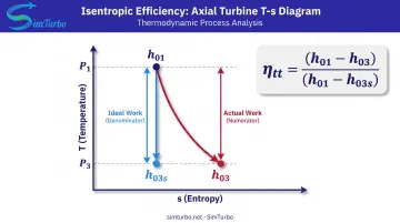
Total-to-static form uses the same actual work in the numerator, but the denominator expands to the outlet static pressure instead of outlet total pressure. NASA applies the same actual-vs-ideal work framing in thermodynamic turbine analysis.
Polytropic Efficiency
Polytropic efficiency is an infinitesimal, or "small-stage," efficiency. For multi-stage machines it separates fluid-dynamic losses from thermodynamic reheat effects, so stages and pressure ratios compare more fairly. Isentropic efficiency folds both loss types together, which skews cross-engine comparison as pressure ratio rises.
Typical Efficiency Ranges by Application
Published figures vary with duty, cooling, and which definition is used:
- Aerospace: NASA reported 88.5% for a cooled Energy Efficient Engine turbine and 90.0% thermodynamic efficiency (92.5% under GE's cycle definition) on a two-stage HPT—same machine, different accounting.
- Industrial power: Heavy-duty multi-stage axials often land in the high-80% to low-90% isentropic range at design point; TIT, cooling extraction, and stage count drive the spread.
- Marine / aeroderivative: Compact engines such as the GE LM2500 favor high power density; efficiency is judged near design RPM and falls off quickly off-design.
When you compare vendor or test data, lock the definition (η_tt vs η_ts vs polytropic), cooling credit, and operating point first—otherwise a 2–3 point gap can be bookkeeping, not aerodynamics. Cycle and matching studies in tools such as SimTurbo make that definition choice explicit before you read too much into a single percentage.
Key Factors Affecting Axial Turbine Efficiency
Multiple loss mechanisms reduce the conversion of fluid enthalpy into shaft work. Understanding these factors helps engineers prioritize design improvements.
Aerodynamic Losses
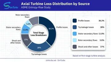
Profile losses result from blade surface friction and flow separation. When flow approaches blades at high incidence angles—common during off-design operation—boundary layers thicken and may separate, increasing entropy generation. An ASME loss-breakdown study assigned 38.2% of audited entropy rise in a first-stage turbine to profile sources.
Secondary flow losses arise from passage vortices and endwall effects. These three-dimensional flow structures redirect energy away from useful work extraction. The same study attributed 11.8% and 5.0% of total loss to stator and rotor secondary flows, respectively.
Shock losses occur in transonic and supersonic stages when local Mach numbers exceed 1.0 on blade surfaces. Shockwaves dissipate kinetic energy and increase entropy, reducing efficiency in high-pressure-ratio stages.
Mechanical and Leakage Losses
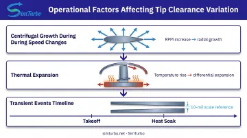
Tip leakage is one of the most significant loss mechanisms. Flow bypasses blade tips through radial clearance gaps between the rotating blades and the stationary casing. NASA research showed that a 10-mil clearance reduction can improve overall mission efficiency by as much as 1% for a common gas-turbine engine.
Clearance varies during operation due to:
- Shaft-speed changes (centrifugal growth)
- Thermal expansion of blades, rotor, case, and shroud
- Transient events like takeoff and heat soak
Disc friction and bearing losses consume shaft power, but they remain small relative to aerodynamic and leakage losses in most modern designs.
Design and Operating Condition Factors
Blade-to-gas speed ratio (velocity ratio) affects how efficiently kinetic energy is extracted. Each turbine design has an optimal velocity ratio that depends on reaction, loading, flow coefficient, and stage architecture. Operating away from this optimum reduces efficiency.
Off-design operation—changes in speed, pressure ratio, mass flow, or inlet temperature—moves the turbine off its design point. Component maps show efficiency falling as operating points leave the peak-efficiency region.
Stage loading (work extraction per stage) influences loss generation. Highly-loaded stages extract more energy per blade row but suffer greater flow turning, higher blade loading, and increased likelihood of separation. Multi-stage designs distribute loading to keep individual stages within efficient operating ranges.
Reynolds number and surface roughness affect boundary layer behavior. A 2018 ASME turbofan low-pressure turbine study found roughness effects significant at takeoff but negligible at cruise. Very rough airfoils increased profile and secondary losses by causing earlier transition and thicker turbulent boundary layers.
How Axial Turbines Achieve High Efficiency
Modern axial turbines combine multiple design strategies to minimize losses and maximize work extraction.
Multi-Stage Pressure Compounding
Dividing total pressure drop across multiple stages keeps gas velocities manageable and reduces aerodynamic losses. The NASA Energy Efficient Engine high-pressure turbine used two stages of moderate loading, balancing efficiency with mechanical complexity.
Optimized Blade Geometry
Blade profiles minimize flow separation and control boundary layer behavior. Key parameters include:
- Airfoil profiles with controlled pressure distributions
- Stagger angles optimized for inlet and exit flow angles
- Twist distributions that account for radial variations in gas velocity
Reaction Ratio
Reaction ratio defines how pressure drop is shared between stationary (stator) and rotating (rotor) blade rows. A 2023 three-stage axial gas-turbine study used 50% reaction at midspan, with approximately equal flow acceleration in stator and rotor. That 50% split is common but not universal. Optimal reaction depends on stage loading, Mach number, and mechanical constraints.
Advanced Cooling Techniques
High-temperature stages need cooling to protect materials without degrading aerodynamic performance. Cooling air carries a thermodynamic penalty, so designs minimize coolant flow while holding metal temperatures within limits.
Tight Tip Clearances and Sealing Systems
NASA defines axial-turbine tip clearance as the radial blade-tip-to-containment gap. Smaller clearances reduce leakage losses but must be large enough to avoid blade rubs. Effective sealing systems, including labyrinth seals, brush seals, and abradable coatings, minimize parasitic flows without mechanical interference.
Optimizing Axial Turbine Efficiency in Design
Engineers use a combination of analytical methods and computational tools to design high-efficiency turbines before building physical hardware.
Meanline and Throughflow Analysis
Meanline models are rapid tools for concept evaluation and off-design prediction. A 2025 equation-oriented method included loss effects in choking and was validated against three single- and multi-stage turbines for mass flow, torque, and exit angle.
NASA's turbo-design tool solves radial-equilibrium equations along streamlines for turbine design, supporting streamline-curvature and throughflow analysis.
These methods establish optimal stage velocity triangles, work distribution, and radial flow variations early in the design process.
Computational Fluid Dynamics (CFD)
CFD enables detailed prediction of three-dimensional flow fields, boundary layers, and loss generation. NASA applied CFD to a two-dimensional blade row from the GE Energy Efficient Engine high-pressure turbine.
In one 2023 ASME air-turbine validation, total-to-total efficiency error was 0.9% for CFD and 1.6% for the meanline model, with stator and rotor loss-coefficient deviations of 5.0% and 1.7%. Errors of that size are model-, mesh-, and operating-point-specific, so teams still treat CFD as a high-resolution check rather than a stand-alone answer.
Multi-Point Optimization
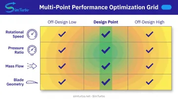
Good efficiency at one design point is not enough. Multi-point optimization checks performance across the map so peak efficiency does not collapse off-design.
Engineers typically vary:
- Rotational speed
- Pressure ratio
- Mass flow
- Blade geometry and stage work split
Performance and matching simulations help screen those points quickly before committing to detailed blade-row aero work.
Blade Clocking
Blade clocking is the circumferential positioning of stator rows relative to upstream wakes. An ASME 1.5-stage cold-air axial-turbine study tested ten positions and tracked how clocking changed the flow field.
Key findings included:
- Shifts in loss generation and energy transport
- Changes in secondary flow and wake interaction
- An optimum position that minimized pressure loss behind the second stator
The team documented effects with pneumatic probes, hot-wire probes, and 3D unsteady viscous calculations.
Measuring and Validating Turbine Efficiency
Accurate efficiency measurement requires careful instrumentation and data reduction.
Experimental Measurement Methods
A 2024 ASME single-stage rig shows what high-accuracy stage testing looks like in practice:
- Inlet total pressure and temperature from six circumferential probes plus radial traverses
- Exit surveys from four full-annulus traversing rakes with Kiel probes and Type-E thermocouples
- Main-gas-path and cooling mass flows on dedicated Venturi flowmeters
- Redundant torque from a torquemeter and dynamometer load cell, plus recorded wheel speed
Reported total-efficiency uncertainty was 0.19–0.32 percentage points, depending on operating condition and sample count.
A QinetiQ engine-scale transonic facility follows the same discipline at engine scale. Its published system covers:
- Mass-flow and direct torque measurement
- Inlet and exit traverses with mass-weighted efficiency
- Calibration procedures and full uncertainty analysis
Computational Simulation
Before hardware is built, CFD is used to predict stage efficiency. Steady runs support design trades; unsteady runs capture wake interactions and secondary flows that steady models miss. Those predictions only hold value when they are checked against measured performance.
System-level tools close that loop. In one documented case, a SimTurbo model of the J85-GE-21 single-spool turbojet matched NASA Lewis Research Center test data within ±2% for thrust, flow rate, temperature, and thrust-specific fuel consumption (TSFC).
That check covers turbine–compressor matching, thermodynamic performance, and operating-point behavior—so engineers can catch efficiency and matching issues before committing to another rig build.
Frequently Asked Questions
How is turbine efficiency calculated?
Turbine efficiency is calculated using the isentropic efficiency formula: η = (h₀₁ - h₀₃) / (h₀₁ - h₀₃s). That is actual enthalpy drop over ideal isentropic enthalpy drop at the same pressure ratio. The subscript "s" marks the isentropic state at the same outlet total pressure.
Why are wind turbines not 100% efficient?
Wind turbines face Betz’s limit (~59.3% theoretical maximum). Axial gas turbines are not 100% efficient either—friction, tip leakage, secondary flows, and non-ideal expansion all leave real losses on the table.
What is the main difference between a radial turbine and an axial turbine?
Axial turbines have flow parallel to the shaft axis, while radial turbines have flow perpendicular to the shaft (radially inward or outward). Axial designs typically achieve higher efficiency in larger power applications due to better aerodynamic control, multi-stage capability, and favorable scaling.
What is considered good efficiency for an axial turbine?
NASA documented aerospace turbines at 88.5% to 92.5% isentropic efficiency, depending on cooling accounting and definition. Modern industrial axial turbines typically reach 85–94%; above 90% is excellent, with results tied to pressure ratio, cooling, and how close the machine runs to design point.
What factors reduce axial turbine efficiency the most?
The biggest losses are tip leakage, blade profile losses, secondary flows, and—in transonic stages—shock losses; their weight shifts with specific speed, loading, and operating point. NASA research showed a 10-mil clearance cut can improve overall mission efficiency by as much as 1% on a common gas-turbine engine.
Can axial turbine efficiency be improved after installation?
Gains after install are limited but real: tip-clearance adjustments, roughness-reducing surface treatments, better seals, and occasional blade-profile work in major overhauls. The highest-ROI path is usually running closer to the design envelope.