Engineers trained on continuous-time control theory often hit a wall converting that math into something a processor can execute every few milliseconds. Get the sampling interval or the integral handling wrong, and a perfectly tuned continuous-time controller becomes unstable in silicon.
This article covers the discrete PID equation, how it's derived from the continuous form, code-level implementation, tuning methods, and the two pitfalls — integral windup and derivative kick — that cause most real-world failures.
Key Takeaways
- Discrete PID computes output at fixed sample intervals T from proportional, integral (summed), and derivative (differenced) terms
- Convert continuous PID to discrete form with forward Euler, backward Euler, or trapezoidal discretization
- Poor sampling rates and unclamped integrators cause most discrete PID instability
- SimTurbo lets engineers test discrete PID and limiter logic on an engine model before hardware runs
What Is a Discrete PID Controller and Why It Matters
A digital controller, whether a PLC, an embedded microcontroller, or a simulated FADEC, can't read a continuous signal. It samples the Process Variable at fixed intervals T and recalculates its output once per cycle.
Everything between samples is invisible to the controller. Texas Instruments notes that this sampling frequency directly caps the range of frequencies a digital controller can meaningfully influence.
The discrete PID formula looks like this:
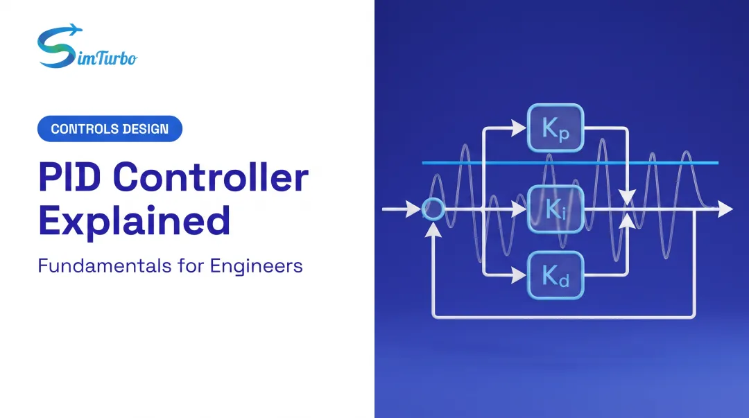
u[k] = Kp·e[k] + Ki·T·Σe[i] + Kd·(e[k] − e[k-1])/T

Where:
- e[k] is the sampled error at step k (setpoint minus feedback)
- T is the sampling interval
- Σe[i] is the running sum of past errors (the integral approximation)
Compare that to bang-bang (ON/OFF) control, which simply flips an actuator fully on or off around a threshold. It's simple, but it causes constant oscillation around the setpoint. That oscillation is unacceptable for a temperature chamber or a turbine shaft-speed loop where smooth, proportional correction matters.
One detail trips people up constantly: T isn't a free variable. Change your sampling interval and your Ki and Kd gains need rescaling, since the integral term scales with T and the derivative term scales inversely with it.
Where Discrete PID Is Used
- Temperature chambers and thermal cycling equipment
- Motor and servo position/speed control
- Tank level and flow regulation
- Gas turbine engine control loops: throttle response, fuel flow scheduling, and shaft speed regulation
That last category is where things get demanding. A gas turbine control law has to hold steady through fast throttle transients without overshooting turbine inlet temperature limits, which is exactly the kind of scenario SimTurbo's component-based engine models are built to test.
Deriving the Discrete Form From the Continuous PID Equation
Start from the standard continuous PID:
u(t) = Kp·e(t) + Ki·∫e(τ)dτ + Kd·de(t)/dt
To make this run on a digital processor, the integral and derivative terms each need a discretization method. There are three common choices:
| Method | Integral Approximation | Notes |
|---|---|---|
| Forward Euler | T(z-1)/z |
Simplest, but can be less stable |
| Backward Euler | Tz/(z-1) |
Most common in embedded systems for numerical stability |
| Trapezoidal (Tustin) | (T/2)(z+1)/(z-1) |
Better frequency matching, but can place poles on the unit circle if applied to an ideal PID without added stabilization |
**Backward Euler is the usual choice in embedded designs** because of its numerical stability margin. Under this method, the integral term becomes a running accumulator multiplied by T, and the derivative becomes a backward difference divided by T:
- Integral:
I[k] = I[k-1] + Ki·T·e[k] - Derivative:
D[k] = Kd·(e[k] − e[k-1])/T

As T shrinks toward zero, the discrete equation converges toward the continuous-time response. A quick step-response comparison at a few sample times makes that convergence easy to see.
One addition almost every real implementation needs: a low-pass filter on the derivative term. Differentiation amplifies high-frequency noise, so an unfiltered derivative on a noisy sensor signal will produce a jittery, unusable output.
Implementing a Discrete PID Controller in Code
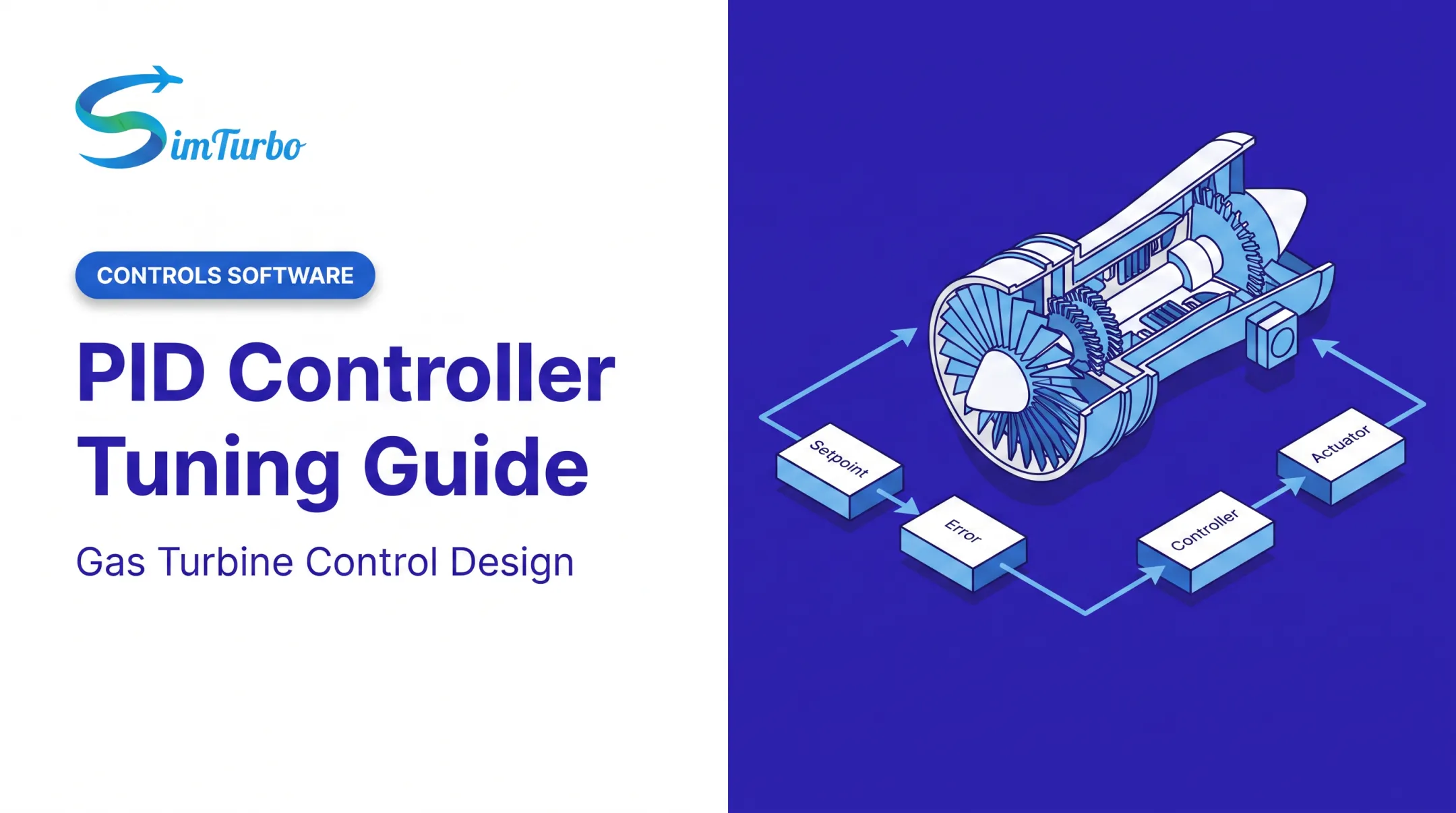
The general structure of any discrete PID update function follows the same five steps:
- Read feedback from the sensor or ADC
- Compute error — setpoint minus feedback
- Calculate P, I, and D terms using the chosen discretization
- Sum the terms for the final output
- Store the current error and output for use in the next cycle

Recursive Form for Embedded Targets
For efficiency on embedded targets, many implementations use the recursive difference-equation form:
u[k] = -a1*u[k-1] - a2*u[k-2] + b0*e[k] + b1*e[k-1] + b2*e[k-2]
This avoids recalculating the integral sum from scratch each cycle and maps cleanly onto fixed-point C code.
Practical Constraints
Three constraints matter more in practice than in theory:
- Output saturation — clamp output to a realistic range (for example ±100% or a PWM duty-cycle limit)
- Fixed loop timing — run the update on a hardware timer interrupt at the same interval T used in your gain calculations
- Numeric format — fixed-point is efficient on small MCUs but needs careful scaling; floating-point is simpler when the hardware supports it
Timing jitter hits the derivative term hardest because that term divides by T. Keep the loop interval strict.
Before any of this touches real hardware, validate the controller against a reference simulation.
SimTurbo lets you exercise discrete PID and limiter blocks on a component-based gas turbine model in real time, then export plant response data to Excel, MATLAB/Simulink, or Python. That cross-check catches gain and anti-windup issues before hardware-in-the-loop migration.
Tuning a Discrete PID Controller
Tuning means selecting Kp, Ki, and Kd (or Ti/Td) while accounting for how T scales the integral and derivative terms. If T is wrong, no amount of gain tuning will fix the loop.
The classic approach, adapted for discrete systems, is the Ziegler-Nichols oscillation method:
- Disable integral and derivative action
- Increase proportional gain until the loop sustains constant-amplitude oscillation
- Record the ultimate gain (Ku) and ultimate period (Tu)
- Apply the standard ratio table
| Controller | Kp | Ti | Td |
|---|---|---|---|
| P | 0.5·Ku | — | — |
| PI | 0.45·Ku | Tu/1.2 | — |
| PID | 0.6·Ku | Tu/2 | Tu/8 |

This method comes from a 1942 ASME paper by Ziegler and Nichols. Use it to get initial gains, then refine against measured overshoot, settling time, and noise sensitivity.
Auto-Tune vs. Manual Fine-Tuning
Modern PLCs and PID tools—including control blocks in simulation platforms such as SimTurbo—often estimate gains through relay-cycle or step tests.
- Auto-tune is useful for a fast first cut on industrial and lab loops
- High-precision or aerospace loops usually need manual trim to hit tight overshoot and settling-time limits
Common Pitfalls: Integral Windup and Derivative Kick
Two failure modes account for most discrete PID instability reports.
Integral windup happens when the accumulated error sum grows excessively large while the Process Variable sits far from setpoint, usually because the actuator is saturated and can't respond fast enough.
The integrator keeps "charging up" even though it has no effect, then causes major overshoot once the actuator finally catches up. Freeze integral accumulation whenever the output is saturated (conditional integration) so the sum cannot wind up unchecked.

Derivative kick is different: a sudden spike in the D-term triggered by an abrupt setpoint change rather than actual process behavior. Because the derivative term reacts to the rate of change of error, a step change in setpoint produces a huge instantaneous spike.
Base the derivative on the feedback signal (measurement) instead of on error so setpoint steps no longer slam the D-term.
Practical safeguards:
- Freeze integral accumulation when the actuator is saturated (conditional integration)
- Compute derivative on measurement, not error, to avoid setpoint-step spikes
- Optionally suspend full PID outside a "controllable region" band around the setpoint until the Process Variable enters that band
That band is common in industrial control and simulation as an extra anti-windup layer when the plant starts far from target.
Frequently Asked Questions
What is the difference between a continuous and discrete PID controller?
Continuous PID computes integrals and derivatives in real time using analog circuitry. Discrete PID samples the error at fixed intervals and approximates those same operations using running sums and finite differences.
How do you calculate a discrete PID controller?
Use u[k] = Kp·e[k] + Ki·T·Σe[i] + Kd·(e[k]-e[k-1])/T as the base formula. The exact coefficients shift depending on whether you use forward Euler, backward Euler, or trapezoidal discretization.
What sampling rate should I use for a discrete PID loop?
Sample fast enough relative to your process dynamics — a common rule of thumb is roughly 10x your fastest time constant. Faster sampling improves derivative accuracy but increases sensitivity to sensor noise.
How do you prevent integral windup in a discrete PID controller?
Common fixes include clamping the output, conditional integration (freezing accumulation during saturation), and controllable-region logic that limits PID action to a band near setpoint.
Can discrete PID controllers be used for gas turbine engine control?
Yes. Turbine control loops for throttle, fuel flow, and shaft speed all run on discrete PID logic. Simulation platforms like SimTurbo include built-in PID and limiter components specifically for validating these control laws before hardware deployment.
What programming languages are used to implement discrete PID controllers?
C/C++ dominates embedded implementations. MATLAB and Python are common for simulation and prototyping. PLC platforms typically use ladder logic or function blocks like Rockwell's PIDE instruction.