Introduction
Gas turbine performance hinges on one critical metric: isentropic efficiency. This dimensionless parameter quantifies how effectively a turbine converts available thermal energy into mechanical work during expansion. Unlike thermal or combustion efficiency, it focuses on the turbine stage itself—the gap between ideal, reversible expansion and real losses from friction, turbulence, and heat transfer.
You rely on it when specifying a turbine for a 100 MW plant, diagnosing an aircraft engine, or sizing marine propulsion. As a design target and an in-service diagnostic, it drives fuel burn, power output, and lifecycle cost.
Real turbines never hit the theoretical 100% mark. Aerodynamic losses, tip clearance leakage, and cooling flows all cut into ideal work. Even a 1% efficiency gain can mean large fuel and emissions savings over years of operation on a utility-scale machine.
This guide defines isentropic efficiency, shows how to calculate it, and explains what moves the number in practice.
Key Takeaways
- Ratio of actual turbine work output to the ideal work from a reversible, constant-entropy expansion
- High-performance aircraft turbines reach 88.5–92.5% at design point, depending on stage design and operating conditions
- Blade aerodynamics, tip clearance, cooling extraction, and Reynolds number effects drive the ideal-to-actual performance gap
- Component-specific metric—separate from cycle thermal efficiency and combustion efficiency
What Isentropic Efficiency Represents in Gas Turbines
Isentropic efficiency (ηT) measures how closely a real turbine approaches ideal, reversible expansion. The mathematical definition is:
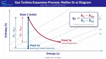
ηT = Wactual / Wisentropic = (h₁ − h₂ₐ) / (h₁ − h₂ₛ)
Where:
- h₁ = inlet enthalpy
- h₂ₐ = actual exit enthalpy
- h₂ₛ = isentropic (ideal) exit enthalpy at the same outlet pressure
This ratio quantifies irreversibility. In an ideal isentropic process, entropy remains constant and all available energy converts to work. Real turbines generate entropy through friction, turbulence, mixing, and heat transfer, raising the actual exit enthalpy and reducing extractable work.
On the h-s (Mollier) diagram, the ideal expansion is a vertical drop from state 1 to state 2s at constant entropy. The actual path bends right as entropy rises, ending at state 2a with higher entropy and higher enthalpy than the ideal exit.
Isentropic efficiency is simply the ratio of those vertical enthalpy drops: (h₁ − h₂ₐ) / (h₁ − h₂ₛ).
Isentropic efficiency is easy to confuse with other common metrics. The table below separates them by what each one measures and where it applies.
| Efficiency Type | What It Measures | Scope |
|---|---|---|
| Isentropic Efficiency | Actual work / ideal work for one component | Single turbine or compressor stage |
| Thermal Efficiency | Net cycle work / heat input | Entire Brayton or Rankine cycle |
| Combustion Efficiency | Actual heat release / fuel chemical energy | Combustor or burner |
| Polytropic Efficiency | Infinitesimal-stage efficiency along expansion path | Useful for comparing turbines across pressure ratios |
Key distinction: Isentropic efficiency is a component-level metric. Thermal efficiency rolls up compressor, combustor, turbine, and heat-exchanger performance across the full cycle. Mixing the two skews test data and performance guarantees.
The Brayton Cycle Context
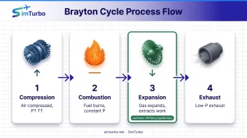
Gas turbines operate on the Brayton cycle, which consists of four processes:
- Compression – Air is compressed adiabatically, raising pressure and temperature
- Combustion – Fuel burns at constant pressure, adding thermal energy
- Expansion – Hot, high-pressure gas expands through the turbine, extracting work
- Exhaust – Low-pressure gas exits to atmosphere or heat recovery
Isentropic efficiency applies specifically to the expansion stage (process 3). Compressor and turbine each have their own isentropic efficiency. This article focuses on turbine expansion, where high-temperature gas drives the shaft and delivers net power.
Typical Range and Operating Boundaries of Isentropic Efficiency
Real-world isentropic efficiency values vary by application, stage design, and operating conditions.
Documented Benchmarks
- NASA/GE Energy Efficient Engine HPT: 90.0% (thermodynamic definition) and 92.5% (GE cycle definition) at design point (1984)
- DLR Aircraft HPT Reconstruction: 88.5% (Pratt & Whitney) to 90.1–91.1% (GE configurations) depending on definition and test conditions (2024)
- Small or older units: Often assumed at 85% in modeling studies—a design assumption rather than measured fleet data
Why Efficiency Shifts in Service
These values are design-point results under specified inlet temperature, pressure ratio, corrected speed, and mass flow. Isentropic efficiency is not a fixed property. It changes with:
- Load condition – Part-load operation shifts the turbine away from its optimal aerodynamic design point
- Ambient conditions – Temperature, pressure, and humidity affect Reynolds number and gas properties
- Component degradation – Erosion, fouling, and thermal distortion degrade blade profiles over time
- Off-design operation – Varying pressure ratios or speeds increase incidence losses and flow separation
Theoretical Boundaries
- Upper limit: 100%, representing a perfectly reversible process with zero entropy generation
- Practical lower threshold: Values below 75–80% typically signal severe degradation or poor operating conditions, where excess fuel burn makes continued operation uneconomical
Key Factors Affecting Isentropic Efficiency in Real-World Operation
The ideal isentropic process assumes reversibility, but real turbines experience multiple sources of irreversibility that degrade efficiency. Each mechanism converts available work into unusable thermal energy.
Aerodynamic Losses: Blade Profile and Secondary Flows
Blade boundary layers, shock waves in transonic stages, and secondary flow vortices near endwalls all dissipate kinetic energy into heat. As flow separates from blade surfaces or generates trailing-edge wakes, the pressure recovery and work extraction suffer.
Key mechanisms:
- Boundary-layer growth on suction and pressure surfaces
- Shock-induced separation at high Mach numbers
- Endwall cross-flows and horseshoe vortices
- Trailing-edge wake mixing
Optimized blade profiles, refined with CFD and rig tests, can cut these losses. How much you gain still depends on baseline geometry, Reynolds number, and Mach regime.
Tip Clearance and Leakage Flows
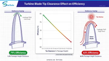
The gap between rotating blade tips and the stationary casing allows high-pressure gas to bypass the blade row without performing useful work. This leakage reduces mass flow through the blade passages and creates tip vortex structures that increase mixing losses.
A 1969 NASA experiment measured static efficiency drop from 0.79 to 0.63 as rotor tip clearance increased from 1.2% to 8.0% of passage height. The relationship was linear over that test range, but the slope still depends on blade design, loading, and Mach number.
Tight clearances matter. Thermal expansion, rotor dynamics, and manufacturing tolerances limit how tightly you can hold them in service.
Cooling Air Requirements
High-pressure turbine blades operate at gas temperatures far exceeding material limits, requiring film cooling or internal convective cooling. Engines extract cooling air from the compressor at high pressure and inject it through blade passages or surface holes.
That cooling air does not fully participate in work extraction. An ASME study of a film-cooled HPT stage found:
- 8.0% efficiency penalty when all mixing and entropy-generation irreversibilities were counted
- 0.7% penalty when unavoidable coolant/mainstream thermal equilibration was excluded from the efficiency definition
The reported cooling penalty depends heavily on accounting convention, cooling mass flow fraction, and injection configuration. Higher turbine inlet temperatures demand more cooling flow, creating a direct trade-off between cycle efficiency and material durability.
Reynolds Number and Scale Effects
Reynolds number (Re) characterizes the ratio of inertial to viscous forces in the flow. Smaller turbines, low-pressure stages, or high-altitude operation reduce Re, thickening boundary layers and increasing viscous dissipation.
A 1959 NASA low-Reynolds-number turbine test found a 5.0 percentage-point loss in peak overall efficiency when Re dropped from 182,500 to 23,000 at design equivalent speed.
Industrial turbines benefit from higher Re through larger size and higher operating pressures. Micro-turbines and UAV engines take steeper viscous penalties.
Component Degradation and Fouling
Over thousands of operating hours, turbine blades experience:
- Erosion from particulate ingestion
- Corrosion from combustion products and contaminants
- Thermal distortion from repeated heating and cooling cycles
- Deposition of combustion residues and airborne contaminants
These effects roughen blade surfaces, alter aerodynamic profiles, and open up tip clearances. An ASME modeling study flagged turbine isentropic-efficiency degradation as the most severe single factor on gas turbine power and efficiency, but it did not publish a universal rate. Maintenance intervals, operating environment, and fuel quality still set how fast that loss builds.
Off-Design Operation and Part-Load Performance
Turbines are optimized for a specific design point defined by inlet temperature, pressure ratio, corrected speed, and mass flow. When operating conditions shift—due to load changes, ambient temperature variation, or altitude—the turbine experiences:
- Incidence losses as flow angles deviate from blade design
- Flow separation when loading exceeds aerodynamic limits
- Mismatch between compressor and turbine operating points
NASA turbine performance maps define efficiency as a function of corrected speed and turbine pressure ratio, with efficiency degrading as the operating point moves away from the design condition. The magnitude of part-load efficiency loss depends on the specific turbine geometry, stage loading, and control strategy.
How Isentropic Efficiency Is Calculated, Measured, and Validated
Isentropic efficiency serves dual roles: as a design prediction tool during development and as an operational performance metric during testing and fleet monitoring. Different calculation and measurement approaches apply in each context.
Calculation for Ideal Gases with Constant Specific Heats
For air-breathing turbines with moderate temperature ranges, a simplified ideal-gas formulation applies:
ηT = (T₁ − T₂ₐ) / (T₁ − T₂ₛ)
Where the isentropic exit temperature is:
T₂ₛ = T₁ × (P₂ / P₁)^((γ−1)/γ)
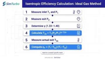
Step-by-Step Calculation:
- Measure or specify inlet total temperature T₁ and total pressure P₁
- Measure or specify exit total pressure P₂
- Determine the specific heat ratio γ (typically 1.33–1.40 for combustion gases)
- Calculate the isentropic exit temperature T₂ₛ using the pressure-ratio equation
- Measure or calculate the actual exit total temperature T₂ₐ
- Compute ηT from the temperature-drop ratio
Limitation: This method assumes constant specific heats, which introduces errors at high temperatures or when gas composition varies significantly.
Calculation Using Real Gas Properties and Steam Tables
For high-temperature gas turbines, steam turbines, or combustion products with variable composition, real gas effects require property tables or equations of state.
Process:
- Determine inlet state: Use measured total pressure P₁ and total temperature T₁ to find inlet enthalpy h₁ and entropy s₁ from NIST REFPROP, JANAF tables, or equivalent databases
- Find isentropic exit enthalpy: At exit pressure P₂, solve for the enthalpy h₂ₛ where entropy s₂ₛ = s₁ (constant-entropy condition)
- Measure actual exit enthalpy: Use measured total pressure P₂ and total temperature T₂ₐ to find h₂ₐ
- Compute efficiency: ηT = (h₁ − h₂ₐ) / (h₁ − h₂ₛ)
Property Resources:
- NIST REFPROP: Helmholtz-energy equations of state for industrially important fluids and mixtures (2022)
- NIST-JANAF Thermochemical Tables: Ideal-gas thermochemical properties for combustion species
Measurement and Instrumentation in Operating Turbines
Field measurement requires calibrated sensors at turbine inlet and exit:
Instrumentation:
- Total pressure probes at turbine inlet (station 3 or 4) and exit (station 4 or 5)
- Total temperature rakes with multiple thermocouples to capture spatial variation
- Mass flow rate measurement (optional for energy-balance validation, cancels from specific-enthalpy ratio)
Procedure:
- Conduct a spatial survey at inlet and exit to capture radial and circumferential profiles
- Mass-average the measurements to obtain representative inlet and exit states
- Use thermodynamic relations (ideal gas or real property tables) to compute ηT
- Correct for measurement bias, probe disturbances, and spatial non-uniformity
Uncertainty: Propagated errors from pressure transducers, thermocouples, property models, and spatial averaging produce test-specific uncertainties. No universal ±2–3% value applies across all installations.
Validation Through Simulation and Modeling
Computational fluid dynamics (CFD) and thermodynamic cycle simulation tools model both isentropic and real expansion processes, enabling engineers to predict efficiency before hardware testing.
Simulation Approaches:
- CFD: Solves Navier-Stokes equations on blade-resolved meshes, capturing boundary layers, shock waves, and secondary flows; predicts entropy generation and work extraction
- Cycle simulation: Uses component maps, empirical loss correlations, and thermodynamic state equations to model engine performance across operating conditions
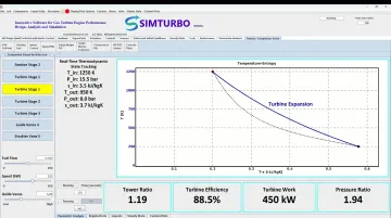
Specialized platforms turn these methods into interactive design tools. SimTurbo, for example, visualizes expansion processes on temperature-entropy and pressure-volume diagrams in real time. Engineers and students can watch how transient events (throttle changes, compressor stall, or sensor failures) affect turbine work extraction and cycle performance.
Its component-based architecture lets users configure compressors, turbines, combustors, nozzles, and control elements, then examine how design changes influence efficiency. The platform applies industry-standard thermodynamic relations, real-gas effects, and component maps. J85-GE-21 validation matched NASA test data within ±2% for thrust, flow rate, temperature, and thrust-specific fuel consumption.
Standards and Best Practices
ASME PTC 22-2023 (Gas Turbines) and ISO 2314:2009 (Gas Turbines – Acceptance Tests) are whole-machine acceptance and performance standards. They specify:
- Test conditions and reference-condition corrections
- Instrumentation requirements and calibration protocols
- Calculation methods for corrected power, heat rate, and thermal efficiency
- Reporting formats for acceptance test results
Important Note: These standards focus on whole-engine performance outputs (power, heat rate, exhaust properties). They do not prescribe a universal method for determining turbine-stage isentropic efficiency. Contract-specific test plans and instrumentation arrangements are required for component-level efficiency measurement.
Operating Implications and Common Misinterpretations
Consequences of Below-Target Isentropic Efficiency
Reduced isentropic efficiency has direct thermodynamic consequences:
Immediate Effects:
- Lower work extraction leaves more thermal energy in the exhaust, raising exhaust gas temperature (EGT) and stressing downstream components
- At fixed fuel flow and inlet conditions, lower ηT reduces shaft work and net power
- More fuel is required per unit of power output; small efficiency losses compound over millions of operating hours
At the system level, an ASME study identified turbine isentropic-efficiency degradation as the most severe individual fault affecting gas turbine power and thermal efficiency. The study did not publish a universal sensitivity factor, but turbine efficiency degradation still disproportionately harms overall plant performance.
Operational Risks:
- Violation of emissions guarantees due to altered combustion conditions
- Shortened inspection intervals as elevated exhaust temperatures accelerate component aging
- Reduced operational flexibility as efficiency losses limit load-following capability
Common Misinterpretations in Engineering Practice
Misinterpretation 1: Universal Design-Point Values
Datasheets report nominal isentropic efficiency at a single design point—specific inlet temperature, pressure ratio, corrected speed, and mass flow. Engineers sometimes apply these values universally across all operating conditions.
Reality: Efficiency varies with load, ambient conditions, and degradation state. NASA turbine performance maps show efficiency as a function of corrected speed and pressure ratio. Off-design operation reduces efficiency as flow angles deviate from blade design and aerodynamic loading changes.
Misinterpretation 2: Confusing Isentropic and Polytropic Efficiency
Polytropic efficiency normalizes performance across pressure ratios by treating the expansion as a series of infinitesimal stages with constant dissipation rate. It is useful for comparing turbines of different sizes or configurations.
Reality: Isentropic efficiency is stage- or component-specific, defined between two thermodynamic states at a given pressure ratio. Polytropic efficiency and isentropic efficiency are not numerically interchangeable and serve different analysis purposes.
Misinterpretation 3: Ignoring Altitude and Climate Corrections
Laboratory or sea-level test data are sometimes applied directly to high-altitude aircraft or hot-climate installations without corrections.
Reality: Reynolds number, gas density, and inlet temperature all affect turbine performance. Acceptance test standards (PTC 22, ISO 2314) specify reference-condition corrections for whole-engine results. Component-level efficiency still requires separate Reynolds-scaling and aerodynamic corrections based on test-specific conditions.
Conclusion
Isentropic efficiency is the governing performance parameter for turbine expansion processes, linking thermodynamic ideality to real work extraction and fuel economy. If you design aircraft engines, diagnose power-plant degradation, or teach gas turbine thermodynamics, this metric shapes both analysis and operating decisions.
Achieving high isentropic efficiency requires careful attention to blade aerodynamics, manufacturing tolerances, cooling strategies, and operating conditions. Even small gains, such as cutting tip clearance by 0.5% or refining cooling-hole placement, produce meaningful lifecycle cost savings across thousands of operating hours and large engine fleets.
Modern simulation tools continue to advance the field. Platforms like SimTurbo help engineers and students visualize expansion processes in real time, compare design-point predictions against transient behavior, and validate control strategies before hardware testing. Research continues to push efficiency higher with additive manufacturing, advanced cooling, and computational optimization. NASA sensitivity studies have explored HPT efficiencies up to 95%, though those levels remain aspirational rather than commercially routine.
Frequently Asked Questions
What is isentropic efficiency?
Isentropic efficiency is the ratio of actual turbine work output to the ideal work output from a reversible, adiabatic (constant-entropy) expansion between the same inlet state and outlet pressure.
How do you calculate the isentropic efficiency of a gas turbine?
From measured inlet P and T, get h₁ and s₁. Find isentropic exit enthalpy h₂ₛ at the exit pressure with s₂ₛ = s₁, then get actual exit enthalpy h₂ₐ. Compute ηT = (h₁ − h₂ₐ) / (h₁ − h₂ₛ); for ideal gases with constant cp, use the equivalent temperature-ratio form.
How do you calculate the efficiency of a gas turbine?
Without a qualifier, "efficiency" usually means thermal efficiency: net cycle work divided by heat input. Isentropic efficiency rates a single component against its ideal reversible process; combustion efficiency tracks how completely fuel is oxidized.
What is the difference between isentropic efficiency and thermal efficiency?
Isentropic efficiency measures how closely a single component (turbine or compressor) approaches ideal, reversible behavior. Thermal efficiency measures the overall cycle's conversion of heat input into net work output, aggregating compressor, combustor, turbine, and heat-exchanger performance. Thermal efficiency is the product of multiple component efficiencies and cycle losses.
What is a typical isentropic efficiency for modern gas turbines?
Aircraft high-pressure turbines typically reach 88.5–92.5% at design point, depending on definition and test conditions. Industrial, older, or smaller machines vary more widely—always confirm efficiency definition, station convention, and reference conditions when comparing values.
Why is isentropic efficiency always less than 100%?
100% efficiency would require a perfectly reversible process with zero entropy generation. All real turbines experience irreversibilities from blade-surface friction, turbulence, tip leakage, cooling-air mixing, and heat transfer. These mechanisms convert available work into unusable thermal energy, raising exit entropy and reducing extractable work below the isentropic ideal.