Transient simulation is time-dependent analysis that captures how systems evolve continuously, solving differential equations that track rates of change, feedback loops, and dynamic response. Unlike steady-state methods that assume equilibrium, transient tools model the path—startup sequences, throttle slams, control-system oscillations, and transient temperature peaks that may exceed steady operation by 15% or more.
This article covers:
- What transient simulation is and how it differs from steady-state analysis
- When to choose transient over steady-state approaches
- Gas turbine applications where transient modeling is essential
- Numerical methods and best practices for accurate, efficient results
Key Takeaways
- Transient simulation tracks time-dependent system evolution, capturing dynamics that steady-state analysis misses
- Use it when response time, peak excursions, control stability, or path-dependent behavior affects design decisions
- Gas turbine design demands transient analysis for startup, shutdown, acceleration, surge events, and controller validation
- Transient runs cost 2-50× more than steady-state but pay off when timing, stability, or peak limits drive requirements
What is Transient Simulation?
Transient simulation (also called time-dependent or unsteady simulation) models how physical systems change over time by solving equations with explicit time derivatives.
Instead of a single equilibrium state, transient methods step forward through time, updating pressures, temperatures, velocities, and other variables at each instant.
Mathematical Foundation
Transient simulations solve differential equations of the form:
∂u/∂t = F(u, t)
The rate of change matters, not just the initial and final states. In gas turbines, that covers shaft acceleration from torque imbalance, pressure changes from mass storage in component volumes, and temperature evolution from heat transfer and combustion dynamics.
What Transient Simulation Captures
Transient methods reveal behaviors invisible to steady-state analysis:
- Time lags between control inputs and system response
- Rates of change such as temperature ramp rates or acceleration times
- Feedback loops in closed-loop control systems
- Oscillations and overshoot that may destabilize operation
- Time-to-equilibrium for startup or load changes
- Peak transient values above steady-state levels (key for thermal and mechanical design)
Example: Consider a water reservoir fed by seasonal rainfall. Steady-state analysis tells you the average water level; transient simulation shows whether the reservoir overflows during spring floods or runs dry in summer droughts. The timing and peaks matter, not just the annual average.
Where Transient Modeling is Essential
Common uses include:
- Computational fluid dynamics (CFD): Unsteady flows, vortex shedding, turbulence
- Heat transfer: Thermal cycling, quenching, transient conduction
- Power systems: Grid stability, fault response, load changes
- Control systems: PID tuning, stability analysis, actuator response
- Gas turbine performance: Startup, acceleration, surge, control validation
Transient vs. Steady-State Simulation: Understanding the Fundamental Difference
Steady-state assumes the system has reached equilibrium, where conditions no longer change with time. Inputs equal outputs; storage terms vanish. It is ideal for final operating conditions: cruise thrust, thermal limits at sustained power, or efficiency at a design point.
Transient simulation captures the full time evolution. It tracks:
- How quickly systems respond
- Intermediate peaks, overshoots, or instabilities
- Path-dependent behavior where history matters
- Dynamic interactions that steady-state methods cannot represent
| Dimension | Steady-State | Transient |
|---|---|---|
| Computational Cost | Baseline | 2–50× longer (duration, time step, physics) |
| Accuracy Requirements | Final equilibrium only | Timing, trajectory, peaks, and final state |
| Data Outputs | Single solution snapshot | Time-series histories for all variables |
| Typical Use Cases | Design-point performance, sustained thermal limits, concept screening | Startup/shutdown, control design, cyclic loads, safety and certification transients |
| Skill Level Required | Moderate | Higher: time-step selection, initial conditions, convergence monitoring |
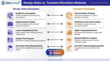
A 2022 CFD study of stirred tanks found that a steady Mean Age Theory method used just 8% of the CPU time of its fully transient counterpart. In that case, transient analysis cost about 12× more.
A gas turbine makes the practical gap clear.
Steady-state: Analyzing cruise power gives sustained turbine-inlet temperature for thermal-limit checks.
Transient: Acceleration from idle to takeoff shows whether the compressor operating line nears surge, how fast the controller responds, and whether temperature spikes exceed blade limits. Steady-state cannot predict those behaviors.
Most projects start with steady-state for design-space exploration and baseline performance, then use transient analysis on critical scenarios such as emergency shutdowns, fault responses, or dynamic load changes.
Use steady-state if:
- You only need final temperatures, pressures, or efficiencies at equilibrium
- Design-point performance is enough for the decision
Use transient if:
- You care about response time, control stability, or transient peaks
- Requirements mention overshoot, settling time, or dynamic behavior
- Certification or safety work involves time-dependent events
When to Use Transient Simulation: Making the Right Engineering Decision
Scenarios Where Transient Simulation is Necessary
Run transient analysis when time history drives the answer:
- Startup and shutdown sequences — ignition, spool-up, coast-down, thermal cycling
- Control design and validation — PID tuning, FADEC logic, actuator response, closed-loop stability
- Cyclic or time-varying loads — load rejection, throttle transients, power cycling
- Safety analysis of short-lived events — surge, flameout, shaft failure, sensor faults
- Certification with time-dependent criteria — FAA 14 CFR 33.73 requires turbine engines to accelerate from minimum to rated takeoff power within 5 seconds under specified conditions
Scenarios Where Steady-State is Sufficient
Steady-state is enough when the operating point holds still long enough to matter:
- Early design exploration and concept screening
- Performance at stable points (cruise, max continuous power)
- Thermal analysis under sustained conditions
- High-level comparison of design alternatives
Cost-Benefit Analysis
Transient runs cost more engineer time and compute than steady-state. Pay that cost only when it maps to a concrete need:
- A hard response-time requirement (for example, response time under 3 seconds)
- Pre-test validation before hardware runs
- Certification rules that demand time-dependent analysis
- Safety margins on peak loads or temperatures
When to Run Both
Most programs should sequence the two methods rather than pick only one:
- Use steady-state to narrow the design space and set baseline performance
- Run transient analysis on one or two finalist designs or critical scenarios
- Validate transient predictions against test data when you have it
Red Flags That Demand Transient Analysis
If requirements call out any of the following, plan on transient work:
- Response time
- Stability
- Overshoot
- Settling time
- Dynamic behavior
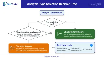
The same rule applies when regulatory tests use time-dependent conditions, such as FAA Part 33 acceleration cycles. In those cases, transient simulation is mandatory.
Transient Simulation in Gas Turbine Engine Design
Why Gas Turbines Are Inherently Transient Systems
Gas turbine engines exhibit time-dependent behavior driven by:
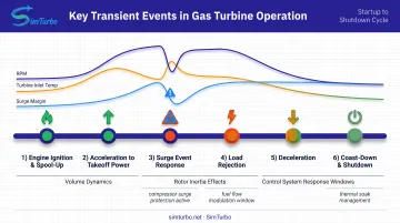
- Rotor inertia: Shaft acceleration follows d(ω)/dt = [W_turbine - W_compressor - W_friction]/(J·ω). Turbine and compressor powers do not balance instantly
- Volume dynamics: Inlet and outlet mass flows differ during transients, so fluid stored in component volumes creates pressure and temperature lags
- Combustion response: Fuel flow changes create delayed heat-release dynamics
- Control system interactions: FADEC logic, actuators, and sensors introduce feedback loops and time delays
Steady-state analysis cannot capture these coupled dynamics.
Key Transient Scenarios in Turbine Design
Critical events requiring transient modeling include:
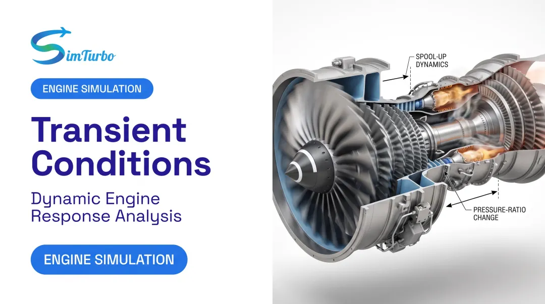
- Engine acceleration (spool-up): Rotor inertia delays speed response; compressor operating line shifts toward surge
- Deceleration and load rejection: Turbine torque imbalance drives rapid speed changes
- Surge events: Compressor stall triggered by rapid throttle movement or inlet distortion
- Transient temperature excursions: Peak turbine-inlet temperatures during acceleration may exceed steady-state values, determining component life
SimTurbo's Transient Simulation Approach
Modeling those events needs time-domain tools, not steady-state maps alone. SimTurbo runs real-time transient simulation on standard PCs with a component-based architecture. Engineers can model:
- Startup and shutdown sequences, including single-spool turbojet startup transients
- Throttle changes, slam-acceleration, and deceleration
- Compressor stall and surge events with control-system response
- Actuator dynamics, sensor failures, and FADEC logic validation
The platform updates time-history graphs, component maps, and thermodynamic-cycle diagrams as conditions change. Engineers can watch RPM, turbine-inlet temperature, and surge margin evolve in real time.
Transient data (RPM, exhaust gas temperature (EGT), thrust, and specific fuel consumption (SFC)) exports to CSV or Excel for post-processing.
Example application: Validate PID performance during rapid throttle changes. Transient runs show whether the controller holds surge margin above 5%, limits turbine-inlet temperature, and meets the required response time for certification and safe operation.
SimTurbo's J85-GE-21 model has been validated against NASA Lewis Research Center test data with accuracy within ±2% for thrust, flow rate, temperature, and TSFC for both steady-state and transient predictions.
Types of Transient Simulation Approaches
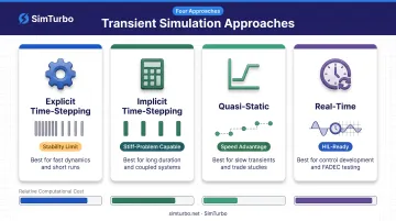
Transient studies are not one-size-fits-all. The right method depends on how fast the dynamics are, how long you need to run, and whether the model must stay in lockstep with hardware or a control law.
Explicit Time-Stepping Methods
Characteristics:
- Updates states directly without solving implicit equations
- Lower cost per time step
- Needs small steps for stability (limits set by the fastest dynamics, such as shaft or volume packing)
Best for:
- Fast dynamics over short run times
- Sharp nonlinear events where tiny stable steps are acceptable
- Capturing rapid spool acceleration, surge onset, or fuel-step response
Implicit Time-Stepping Methods
Characteristics:
- Solves the system iteratively at each time step
- Supports larger steps and stronger stability on stiff problems
- Higher cost per step, usually fewer steps overall
Best for:
- Long-duration engine runs
- Stiff systems with split time scales (fast combustion vs. slow thermal soak)
- Coupled shaft, thermal, and control-loop behavior in one model
Quasi-Static Simulation
Characteristics:
- Approximates slow transients as a sequence of steady-state solutions
- Assumes equilibrium at each step
- Much faster than full transient, but drops fast dynamics
Best for:
- Slow load or setpoint changes where sub-step dynamics are negligible
- Mission or operating-line sweeps over long timelines
- Early architecture trade studies before full dynamic fidelity is required
Real-Time Simulation
Characteristics:
- Tuned to run at wall-clock speed
- Syncs with physical hardware for hardware-in-the-loop (HIL) testing
- May trade some fidelity for guaranteed execution speed
Best for:
- Control system development and FADEC integration
- Testing physical controllers against a simulated plant
- Operator training and control-law validation before rig or engine test
Choose explicit methods when you must resolve the fastest events, implicit when stiffness or run length dominates, quasi-static when only the slow envelope matters, and real-time when the model has to keep pace with hardware or a live controller.
Common Challenges and Best Practices in Transient Simulation
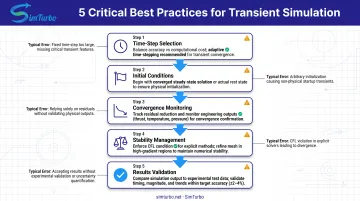
Getting useful transient results means managing accuracy, run time, and physical credibility at once. The practices below address the failure modes that most often skew timing, peaks, or convergence.
Time-Step Selection
Challenge: Balancing accuracy (small steps) vs. computational cost (large steps).
Best practices:
- Base time-step resolution on the fastest relevant physical or control time scale
- Use adaptive time-stepping when available: smaller steps around rapid changes, larger steps in slowly varying regions
- Validate temporal discretization by repeating the simulation with a smaller time step and comparing results
Initial Conditions
Challenge: Transient simulations are sensitive to starting conditions.
Best practices:
- When the transient begins at an established operating point, start from a converged steady-state solution to improve convergence and reduce initialization artifacts
- When modeling startup from rest, use the actual initial state (e.g., ambient temperature, zero speed)
- Document and validate initial-condition assumptions
Validating Transient Results
Challenge: Ensuring transient predictions are physically accurate.
Best practices:
- Compare transient simulation results to experimental data or analytical solutions when possible
- Validate both timing (when events occur) and magnitude (peak values)
- NASA reported 1-2% gas-generator-speed error in one transient comparison; a 2025 ASME shaft-failure model predicted terminal turbine speed within 4%
- Check residual reduction within each time step and monitor convergence of engineering outputs
Explicit Stability and CFL Condition
Challenge: Explicit methods require very small time steps to remain stable.
Best practices:
- Ensure the stress wave does not cross the smallest mesh element in one time step
- Refine mesh in critical regions to avoid driving the global time step too low
Frequently Asked Questions
What is the difference between a transient simulation and a steady-state simulation?
Steady-state assumes equilibrium where conditions no longer change with time; it solves for the final operating point. Transient simulation tracks time-dependent evolution, capturing response dynamics, oscillations, peaks, and the path from one state to another.
What are the three types of simulations?
The three time-behavior classifications are steady-state (equilibrium), transient (time-dependent), and quasi-static (slow transients treated as a series of equilibria). Modal or frequency-domain analysis is sometimes counted as a fourth category but addresses different physics.
Is a transient response good or bad?
Transient response simply describes how a system reacts to change. Engineers design for desired transient behavior: fast response without excessive overshoot, stable settling, and operation within safety limits during dynamic events.
What is an example of a transient response?
A gas turbine accelerating from idle to full power is a clear transient response. Other examples include a car's suspension hitting a bump or indoor temperature shifting when HVAC turns on.